Page 125 - MATLAB an introduction with applications

110 ——— MATLAB: An Introduction with Applications

Solution:
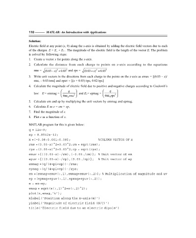
Electric field at any point (x, 0) along the x-axis is obtained by adding the electric field vectors due to each
of the charges. E = E – + E + . The magnitude of the electric field is the length of the vector E. The problem
is solved by following steps:
1. Create a vector x for points along the x-axis.
2. Calculate the distance from each charge to points on x-axis according to the equations
2
2
2
rms = (0.03– )x + 0.03 and rps = (0.03+ x ) + 0.03 2
3. Write unit vectors in the directions from each charge to the points on the x-axis as emuv = [(0.03 – x)/
rms, – 0.03/rms] and epuv = [(x + 0.03)/rps, 0.02/rps]
4. Calculate the magnitude of electric field due to positive and negative charges according to Coulomb’s
 q   q 
law: E = emmag =   4πε 0 rms  and E + = epmag =   4πε 0 rps 
2 
2 
5. Calculate em and ep by multiplying the unit vectors by emmag and epmag.
6. Calculate E as e = em + ep,
7. Find the magnitude of e.
8. Plot e as a function of x.

MATLAB program for this is given below:
q = 12e–9;
ep = 8.8542e–12;
x =[–0.08:0.001:0.08]; %COLUMN VECTOR OF x
rms =(0.03–x)^2+0.03^2;rm = sqrt(rms);
rps =(0.03+x)^2+0.03^2;rp = sqrt(rps);
.
emuv =[((0.03–x) /rm),(–0.03./rm)]; % Unit vector of em
.
epuv =[((0.03+x) /rp),(0.03./rp)]; % Unit vector of ep
.
emmag =(q/(4*pi*ep)) /rms;
.
epmag =(q/(4*pi*ep)) /rps;
em =[emmag*emuv(:,1),emmag*emuv(:,2)]; % Multiplication of magnitude and uv
ep =[epmag*epuv(:,1),epmag*epuv(:,2)];
e = em+ep;
emag = sqrt(e(:,1)^2+e(:,2)^2);
plot(x,emag,‘k’);
xlabel(‘Position along the x–axis(m)’)
ylabel(‘Magnitude of electric field (N/C)’)
title(‘Electric field due to an electric dipole’)

F:\Final Book\Sanjay\IIIrd Printout\Dt. 10-03-09