Page 287 - Machine Learning for Subsurface Characterization

Classification of sonic wave Chapter 9 249

An extensive validation was performed to ensure the reliability of the simulated
dataset generated using FMM for purposes of developing/evaluating data-
driven models for the noninvasive static characterization of mechanical
discontinuities.

3.2.1 Numerical model of homogeneous material at various
spatial discretization
Discretization governs the accuracy of the FMM and k-Wave simulations [17].
Spatial discretization of a numerical model is defined by the number of grids (or
grid size) implemented in the model. With the increase in the number of girds,
the accuracy and computational time of the simulation of wavefront travel time
will increase till a certain optimal number of grids. Compressional velocity of
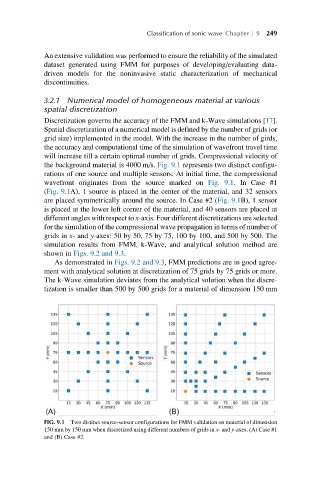
the background material is 4000 m/s. Fig. 9.1 represents two distinct configu-
rations of one source and multiple sensors. At initial time, the compressional
wavefront originates from the source marked on Fig. 9.1. In Case #1
(Fig. 9.1A), 1 source is placed in the center of the material, and 32 sensors
are placed symmetrically around the source. In Case #2 (Fig. 9.1B), 1 sensor
is placed at the lower left corner of the material, and 40 sensors are placed at
different angles with respect to x-axis. Four different discretizations are selected
for the simulation of the compressional wave propagation in terms of number of
grids in x- and y-axes: 50 by 50, 75 by 75, 100 by 100, and 500 by 500. The
simulation results from FMM, k-Wave, and analytical solution method are
shown in Figs. 9.2 and 9.3.
As demonstrated in Figs. 9.2 and 9.3, FMM predictions are in good agree-
ment with analytical solution at discretization of 75 grids by 75 grids or more.
The k-Wave simulation deviates from the analytical solution when the discre-
tization is smaller than 500 by 500 grids for a material of dimension 150 mm

FIG. 9.1 Two distinct source-sensor configurations for FMM validation on material of dimension
150 mm by 150 mm when discretized using different numbers of grids in x- and y-axes. (A) Case #1
and (B) Case #2.