Page 289 - Machine Learning for Subsurface Characterization

Classification of sonic wave Chapter 9 251

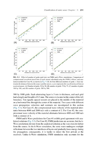
FIG. 9.3 Effect of number of grids (grid size) on FMM and k-Wave simulations. Comparison of
compressional wavefront travel time at each sensor calculated using the FMM, k-Wave, and ana-
lytical method for Case #2, as shown in Fig. 9.1B, for four different numbers of grids. x-Axis rep-
resents the distance between the source and the sensor; y-axis represents the wavefront travel time at
receiver/sensor. (A) Number of grids: 50 by 50, (B) number of grids: 75 by 75, (C) number of grids:
100 by 100, and (D) number of grids: 500 by 500.

500 by 1000 grids. Each alternating layer is 5 mm in thickness, and each grid
had a length and breadth of 0.3 mm. The source is located at the center of the left
boundary. Ten equally spaced sensors are placed in the middle of the material
on a horizontal line through the center of the material. Two cases with different
wave propagation velocities and contrasts are investigated in this section
(Fig. 9.4). For Case #1, the compressional wave velocity of the material alter-
nates between 4000 and 2000 m/s with a contrast of 2. For Case #2, the com-
pressional wave velocity of the material alternates between 4000 and 1000 m/s
with a contrast of 4.
FMM and k-Wave predictions for Case #1 exhibit good agreement with ana-
lytical solutions (Fig. 9.5). For Case #2, FMM predictions are accurate, but the k-
Wave predictions deviate from the analytical solution as the wave travels farther
from the source. In the k-Wave simulation, the sonic wave undergoes multiple
reflections between the two interfaces of layers and gradually loses energy during
the propagation; consequently, it is harder to detect the first arrivals at the
receivers. Unlike k-Wave simulation, FMM simulation only accounts for the