Page 292 - Machine Learning for Subsurface Characterization

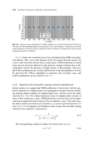
254 Machine learning for subsurface characterization

FIG. 9.6 Source-sensor configuration for FMM validation on a material of dimension 150 mm by
300 mm with 300 embedded parallel discontinuities of 0.3-mm thickness. Compressional velocity
of discontinuities in Case #1 is 45 m/s, and that in Case #2 is 450 m/s. Compressional velocity of the
background material is 4000 m/s.

Fig. 9.7 shows the wavefront travel time calculated using FMM and analyt-
ical solution. The x-axis is the distance of the 10 sensors from the source; the
y-axis is the wavefront arrival time at each sensor. FMM predictions of travel
times are not adversely affected by the presence of large contrasts due to dis-
continuities and by the presence of high density of discontinuity. However,
the k-Wave predictions are severely affected due to the discontinuities of Case
#1 and Case #2. k-Wave simulation is extremely slow for these cases, and
k-Wave predictions are not added to Fig. 9.7.

3.2.4 Material with smoothly varying velocity distribution
In this section, we compare the FMM predictions of travel time with the ana-
lytical solutions for compressional wave propagation through materials exhibit-
ing smooth spatial variation of compressional wave velocity across the entire
material (Fig. 9.8). For certain functional forms of compressional velocity in
terms of the coordinates x and y, FMM predictions of travel time can be repre-
sented in an analytical form in terms of the coordinates x and y. For such cases,
the arrival of the wavefront at any location (x, y) can be expressed in terms of x
and y (Fig. 9.9). For purposes of validation, in this section, the smoothly varying
velocity of the material is expressed as

1
(9.3)
0:5
f ¼
2 2
ð 2xÞ + 2yð Þ
The corresponding analytical solution for arrival time t(x,y)is
2
t ¼ x + y 2 (9.4)