Page 296 - Machine Learning for Subsurface Characterization

258 Machine learning for subsurface characterization

The receivers are referred using indices ranging from 0 to 27. The receivers
located on the upper boundary adjacent to the source-bearing boundary have
index ranging from 0 to 9. The receivers located on the lower boundary adjacent
to the source-bearing boundary have index ranging from 18 to 27. The receivers
located on the boundary opposite to the source-bearing boundary have index
ranging from 9 to 18. On each of the three boundaries, the receivers are placed
incrementally in the order of indices. The receiver with index of 0 is located at
the top left corner, the receiver with index of 9 is located at the top right corner,
the receiver with index of 27 is located at the bottom right corner, and the
receiver with index of 18 is located at the bottom left corner.
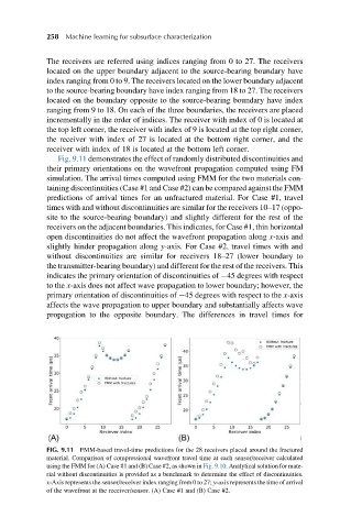
Fig. 9.11 demonstrates the effect of randomly distributed discontinuities and
their primary orientations on the wavefront propagation computed using FM
simulation. The arrival times computed using FMM for the two materials con-
taining discontinuities (Case #1 and Case #2) can be compared against the FMM
predictions of arrival times for an unfractured material. For Case #1, travel
times with and without discontinuities are similar for the receivers 10–17 (oppo-
site to the source-bearing boundary) and slightly different for the rest of the
receivers on the adjacent boundaries. This indicates, for Case #1, thin horizontal
open discontinuities do not affect the wavefront propagation along x-axis and
slightly hinder propagation along y-axis. For Case #2, travel times with and
without discontinuities are similar for receivers 18–27 (lower boundary to
the transmitter-bearing boundary) and different for the rest of the receivers. This
indicates the primary orientation of discontinuities of 45 degrees with respect
to the x-axis does not affect wave propagation to lower boundary; however, the
primary orientation of discontinuities of 45 degrees with respect to the x-axis
affects the wave propagation to upper boundary and substantially affects wave
propagation to the opposite boundary. The differences in travel times for

FIG. 9.11 FMM-based travel-time predictions for the 28 receivers placed around the fractured
material. Comparison of compressional wavefront travel time at each sensor/receiver calculated
using the FMM for (A) Case #1 and (B) Case #2, as shown in Fig. 9.10. Analytical solution for mate-
rial without discontinuities is provided as a benchmark to determine the effect of discontinuities.
x-Axis represents the sensor/receiver index ranging from 0 to 27; y-axis represents the time of arrival
of the wavefront at the receiver/sensor. (A) Case #1 and (B) Case #2.