Page 436 - Marks Calculation for Machine Design

P2: Sanjay
P1: Shibu/Rakesh
January 4, 2005
15:34
Brown˙C10
Brown.cls
APPLICATION TO MACHINES
418
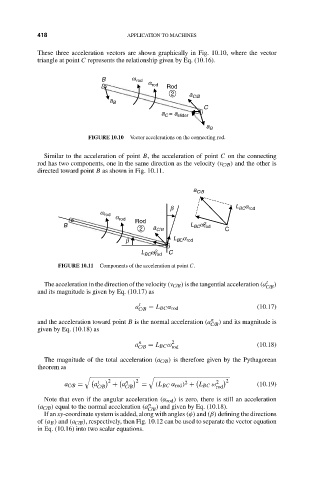
These three acceleration vectors are shown graphically in Fig. 10.10, where the vector
triangle at point C represents the relationship given by Eq. (10.16).
B w rod
a rod Rod
2 a C/B
a B
C
a = a slider
C
a B
FIGURE 10.10 Vector accelerations on the connecting rod.
Similar to the acceleration of point B, the acceleration of point C on the connecting
rod has two components, one in the same direction as the velocity (v C/B ) and the other is
directed toward point B as shown in Fig. 10.11.
a C/B
a
b L BC rod
w rod
a rod
w
2
B Rod L BC rod
2 a C/B C
a
b L BC rod
L BC w 2 rod C
FIGURE 10.11 Components of the acceleration at point C.
The acceleration in the direction of the velocity (v C/B ) is the tangential acceleration (a t )
C/B
and its magnitude is given by Eq. (10.17) as
a t (10.17)
C/B = L BC α rod
n
and the acceleration toward point B is the normal acceleration (a C/B ) and its magnitude is
given by Eq. (10.18) as
a n = L BC ω 2 (10.18)
C/B rod
The magnitude of the total acceleration (a C/B ) is therefore given by the Pythagorean
theorem as

t 2 n 2 2 2 2
a C/B = a + a = (L BC α rod ) + L BC ω (10.19)
C/B C/B rod
Note that even if the angular acceleration (α rod ) is zero, there is still an acceleration
(a C/B ) equal to the normal acceleration (a n ) and given by Eq. (10.18).
C/B
If an xy-coordinate system is added, along with angles (φ) and (β) defining the directions
of (a B ) and (a C/B ), respectively, then Fig. 10.12 can be used to separate the vector equation
in Eq. (10.16) into two scalar equations.