Page 437 - Marks Calculation for Machine Design

P2: Sanjay
P1: Shibu/Rakesh
15:34
January 4, 2005
Brown.cls
Brown˙C10
MACHINE MOTION
y
a C/B b 419
B
L AB w 2 crank
L BC rod
a
f
L BC w 2 rod C
f L AB crank b
a
a B
x
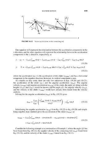
FIGURE 10.12 Vector accelerations on the connecting rod.
One equation will represent the relationship between the acceleration components in the
x-direction, and the other equation will represent the relationship between the acceleration
components in the y-direction, respectively, as
2 2
x: −a C =−L AB ω sin φ + L AB α crank cos φ − L BC ω cos β + L BC α rod sin β
crank rod
(10.20)
2 2
y: 0 =−L AB ω cos φ − L AB α crank sin φ + L BC ω sin β + L BC α rod cos β
crank rod
(10.21)
where the acceleration (a C ) is the acceleration of the slider (a slider ) and has a horizontal
component in the negative direction; however, its vertical component is zero.
As complex as they seem, there are only two unknowns in Eqs. (10.20) and (10.21),
the acceleration of the slider (a C ) and the angular acceleration (α rod ). The angular
velocity (ω crank ) and angular acceleration (α crank ) of the crank, the angle (φ) along with the
lengths (L AB ) and (L BC ) would be known, and the angle (β), the angular velocity (ω rod ),
and the velocity of the slider (v slider ) would have already been found from the velocity
analysis.
Solving for the angular acceleration (α rod ) in Eq. (10.21) gives

2
L AB ω crank cos φ + α crank sin φ 2
α rod = − ω rod tan β (10.22)
L BC cos β

Substituting the angular acceleration (α rod ) from Eq. (10.22) to Eq. (10.20) and simpli-
fying (algebra steps omitted) gives the acceleration of the slider (a slider ) as

2
a slider = L AB ω (sin φ − cos φ tan β) − α crank (cos φ + sin φ tan β)
crank
(10.23)
+ L BC ω 2 (cos β + tan β sin β)
rod
Consider the following example as a continuation of Example 1, where the angle (β) has
been found from Eq. (10.12), the angular velocity of the connecting rod (ω rod ) found from
Eq. (10.10), and the velocity of the slider (v slider ) found from Eq. (10.11).