Page 211 - Materials Science and Engineering An Introduction

6.6 Tensile Properties • 183

500
70
Tensile strength
450 MPa (65,000 psi)
60
400

3
A 10 psi 50
40
MPa
300
Stress (MPa) 200 30 40 Stress (10 3 psi)
Yield strength
200 250 MPa (36,000 psi) 30
20
100 20
10
100
10
0 0
0 0.005
0 0
0 0.10 0.20 0.30 0.40
Strain
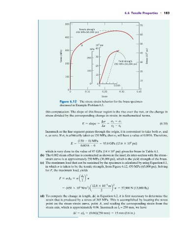
Figure 6.12 The stress–strain behavior for the brass specimen
discussed in Example Problem 6.3.

this computation. The slope of this linear region is the rise over the run, or the change in
stress divided by the corresponding change in strain; in mathematical terms,

s s 2 - s 1
E = slope = = (6.10)
P P 2 - P 1
Inasmuch as the line segment passes through the origin, it is convenient to take both s 1 and
P 1 as zero. If s 2 is arbitrarily taken as 150 MPa, then P 2 will have a value of 0.0016. Therefore,
(150 - 0) MPa
6
E = = 93.8 GPa (13.6 * 10 psi)
0.0016 - 0
6
which is very close to the value of 97 GPa (14 * 10 psi) given for brass in Table 6.1.
(b) The 0.002 strain offset line is constructed as shown in the inset; its inter-section with the stress–
strain curve is at approximately 250 MPa (36,000 psi), which is the yield strength of the brass.
(c) The maximum load that can be sustained by the specimen is calculated by using Equation 6.1,
in which s is taken to be the tensile strength, from Figure 6.12, 450 MPa (65,000 psi). Solving
for F, the maximum load, yields
2
d 0
F = sA 0 = s a b p
2
-3
12.8 * 10 m 2
6 2
= (450 * 10 N/m ) a b p = 57,900 N (13,000 lb f )
2
(d) To compute the change in length, ≤l, in Equation 6.2, it is first necessary to determine the
strain that is produced by a stress of 345 MPa. This is accomplished by locating the stress
point on the stress–strain curve, point A, and reading the corresponding strain from the
strain axis, which is approximately 0.06. Inasmuch as l 0 = 250 mm, we have

l = Pl 0 = (0.06)(250 mm) = 15 mm (0.6 in.)