
Page 265 - Mechanical design of microresonators _ modeling and applications
P. 265
0-07-145538-8_CH05_264_08/30/05
Resonant Micromechanical Systems
264 Chapter Five
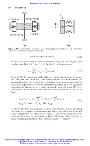
x
actuation beam-spring k
x Fcf c
m m
beam-spring sensing
k
(a) (b)
Figure 5.41 Electrostatic actuation and beam-spring suspension: (a) schematic
microdevice; (b) lumped-parameter model.
mx ˙˙ + cx ˙ +2kx = F sin (Ȧt) (5.92)
0
where it is assumed that the electrostatic force F cf varies according to a sine
law. By using Eqs. (5.91) and (1.13), Eq. (5.92) is reformulated as
2
Ȧ z F 0
r 0
2
x ˙˙ + + Ȧ x = sin (Ȧt) (5.93)
ʌȝx ˙ r m
Equation (5.93) is nonlinear as the velocity is in the denominator of the sec-
ond term of the left-hand side. This equation can be used to determine the
average damping ratio by applying a numerical integration scheme, such as
9
the Newmark procedure (see Wood, for instance) which gives two equations
connecting the displacement, velocity, and acceleration of a single-DOF sys-
tem (such as the one studied here) at two consecutive moments in time in the
form:
(ǻt) 2 (ǻt) 2
x = x + ǻtx ˙ + (1 íȕ ) x ˙˙ + ȕ x ˙˙
i+1 i i 2 2 i 2 2 i+1 (5.94)
x ˙ = x ˙ + ǻt(1 íȕ ) x ˙˙ + ǻt ȕ x ˙˙
i+1 i 1 i 1 i+1
In Eqs. (5.94), ¨t is the sampling rate (the time interval between recording
two consecutive capacitive measurements), whereas ȕ 1 and ȕ 2 are numerical
control parameters, for values greater than 0.5, the Newmark scheme is un-
9
conditionally stable, as mentioned by Wood. Equation (5.93) can also be
sampled corresponding to the time stations i and i + 1, namely,
Downloaded from Digital Engineering Library @ McGraw-Hill (www.digitalengineeringlibrary.com)
Copyright © 2004 The McGraw-Hill Companies. All rights reserved.
Any use is subject to the Terms of Use as given at the website.