Page 183 - Mechatronic Systems Modelling and Simulation with HDLs

172 8 MICROMECHATRONICS

If we finally equate (8.13) and (8.14), then using (8.7) and (8.11) we find the
following expression for the stiffness matrix:

T
K = B CBdA (8.15)
A
Because the coordinates of the matrix B are defined in the natural coordinates, the
integration must be performed using these coordinates

dA = det J ds dt (8.16)

Substituting yields:

T
K = F ds dt where F = B CB det J (8.17)
A
Since the analytical integration is difficult to get to grips with, at this point a numer-
ical integration will be performed on the basis of the Gauss–Legendre quadrature.
To this end the following support points are used in natural coordinates:

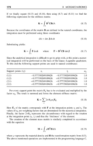
Support points (i,j) s i t j α ij

(1,1) −0.577350269189626 −0.577350269189626 1.0
(1,2) −0.577350269189626 +0.577350269189626 1.0
(2,1) +0.577350269189626 −0.577350269189626 1.0
(2,2) +0.577350269189626 +0.577350269189626 1.0

For every support point the matrix F ij has to be evaluated and multiplied by the
factor α ij . The result is summed and forms the element stiffness matrix:

K = 2πR ij α ij F ij (8.18)
i,j

Here F ij of the matrix corresponds with F at the integration points s i and t j .The
values of α ij are weighting factors that are determined for the numerical integration.
Finally, the factor 2πR ij represents the circumference with regard to the rotation
at the integration point (s i ,t j ) and thus the ‘thickness’ of the element.
The creation of the element mass matrix is similarly completed in accordance
with the equation:

T
M = ρH H dA (8.19)
A
where ρ represents the material density and H the transformation matrix from (8.5).
The above-mentioned operations are implemented in the programming language C.