Page 148 - MODELING OF ASPHALT CONCRETE

126 Cha pte r F i v e

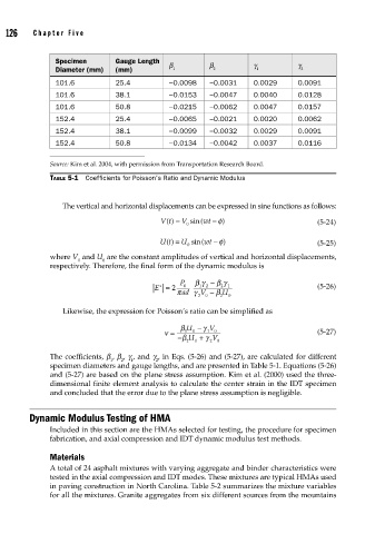
Specimen Gauge Length
b b g g
Diameter (mm) (mm) 1 2 1 2
101.6 25.4 −0.0098 −0.0031 0.0029 0.0091
101.6 38.1 −0.0153 −0.0047 0.0040 0.0128
101.6 50.8 −0.0215 −0.0062 0.0047 0.0157
152.4 25.4 −0.0065 −0.0021 0.0020 0.0062
152.4 38.1 −0.0099 −0.0032 0.0029 0.0091
152.4 50.8 −0.0134 −0.0042 0.0037 0.0116

Source: Kim et al. 2004, with permission from Transportation Research Board.

TABLE 5-1 Coefficients for Poisson’s Ratio and Dynamic Modulus

The vertical and horizontal displacements can be expressed in sine functions as follows:
Vt() = V sin( wt − φ ) (5-24)
0
Ut() = U sin( wt − φ )
0 (5-25)
where V and U are the constant amplitudes of vertical and horizontal displacements,
0 0
respectively. Therefore, the final form of the dynamic modulus is
P βγ − β γ
∗
E = 2 0 1 2 2 1 (5-26)
π ad γ V − β U
2 0 2 0
Likewise, the expression for Poisson’s ratio can be simplified as
β U − γ V
ν = 1 0 1 0 (5-27)
− β U 0 + γ V 0
2
2
The coefficients, b , b , g , and g , in Eqs. (5-26) and (5-27), are calculated for different
1 2 1 2
specimen diameters and gauge lengths, and are presented in Table 5-1. Equations (5-26)
and (5-27) are based on the plane stress assumption. Kim et al. (2000) used the three-
dimensional finite element analysis to calculate the center strain in the IDT specimen
and concluded that the error due to the plane stress assumption is negligible.

Dynamic Modulus Testing of HMA
Included in this section are the HMAs selected for testing, the procedure for specimen
fabrication, and axial compression and IDT dynamic modulus test methods.

Materials
A total of 24 asphalt mixtures with varying aggregate and binder characteristics were
tested in the axial compression and IDT modes. These mixtures are typical HMAs used
in paving construction in North Carolina. Table 5-2 summarizes the mixture variables
for all the mixtures. Granite aggregates from six different sources from the mountains