Page 167 - MODELING OF ASPHALT CONCRETE

Interr elationships among Asphalt Concr ete Stif fnesses 145

Analytical Representation
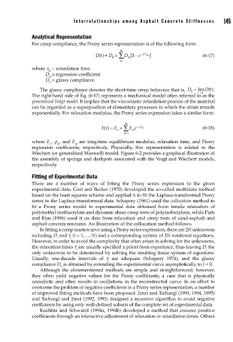
For creep compliance, the Prony series representation is of the following form:
M
Dt () = D + ∑ D [ −1 e − t/τ m ] (6-17)
m
0
m
where t = retardation time
m
D = regression coefficient
m
D = glassy compliance
0
D t)
The glassy compliance denotes the short-time creep behavior, that is, D = lim ( .
0
t→
0
The right-hand side of Eq. (6-17) represents a mechanical model often referred to as the
generalized Voigt model. It implies that the viscoelastic retardation process of the material
can be regarded as a superposition of elementary processes in which the strain retards
exponentially. For relaxation modulus, the Prony series expression takes a similar form:
∞ ∑
Et () = E + M E e − t/ρ m (6-18)
m
m=1
where E , r , and E are long-time equilibrium modulus, relaxation time, and Prony
∞ m m
regression coefficients, respectively. Physically, this representation is related to the
Wiechert (or generalized Maxwell) model. Figure 6-2 provides a graphical illustration of
the assembly of springs and dashpots associated with the Voigt and Wiechert models,
respectively.
Fitting of Experimental Data
There are a number of ways of fitting the Prony series expression to the given
experimental data. Cost and Becker (1970) developed the so-called multidata method
based on the least squares scheme and applied it to fit the Laplace-transformed Prony
series to the Laplace-transformed data. Schapery (1961) used the collocation method to
fit a Prony series model to experimental data obtained from tensile relaxation of
polymethyl methacrylate and dynamic shear creep tests of polyisobutylene, while Park
and Kim (1996) used it on data from relaxation and creep tests of sand-asphalt and
asphalt concrete mixtures. An illustration of the collocation method follows.
In fitting a creep mastercurve using a Prony series expression, there are 2N unknowns
including D and t (i = 1,…, N) and a corresponding system of 2N nonlinear equations.
i i
However, in order to avoid the complexity that often arises in solving for the unknowns,
the relaxation times t are usually specified a priori from experience, thus leaving D the
i i
only unknowns to be determined by solving the resulting linear system of equations.
Usually, one-decade intervals of t are adequate (Schapery 1974), and the glassy
i
compliance D is obtained by extending the experimental curve asymptotically to t = 0.
0
Although the aforementioned methods are simple and straightforward; however,
they often yield negative values for the Prony coefficients, a case that is physically
unrealistic and often results in oscillations in the reconstructed curve. In an effort to
overcome the problem of negative coefficients in a Prony series representation, a number
of improved fitting methods have been proposed. Emri and Tschoegl (1993, 1994, 1995)
and Tschoegl and Emri (1992, 1993) designed a recursive algorithm to avoid negative
coefficients by using only well-defined subsets of the complete set of experimental data.
Kashhta and Schwarzl (1994a, 1994b) developed a method that ensures positive
coefficients through an interactive adjustment of relaxation or retardation times. Others