Page 172 - MODELING OF ASPHALT CONCRETE

150 Cha pte r S i x

{r , E (i = 1,…, m) and E } or {t , D (j = 1,…, n), D and h } are known and the target time
i i e j j j 0
constants specified, the unknown set of constants can be determined through a system
of linear algebraic equations. For example, creep compliance in its Prony series form, D
j
(j 1,…, n), can be determined from relaxation modulus E(t) as follows:
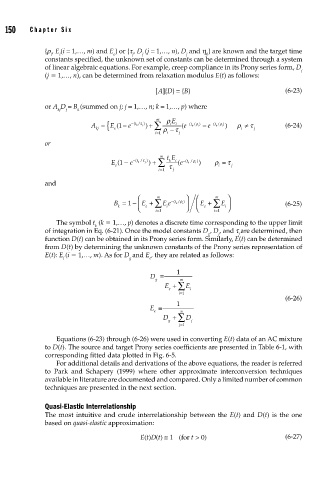
[]{} = { } (6-23)
B
AD
or A D = B (summed on j; j = 1,…, n; k = 1,…, p) where
kj j k
E
m
i
E
A = { (1 − e −(/τ j ) ) + ∑ ρ ρ i − τ e ( −(/ρ i ) i − e − k t ( / )ρ i ) ρ i ≠ τ j (6-24)
t k
t k
e
kj
i=1 i j
or
m
E (1 − e − (/τ j ) ) + ∑ tE i e ( − (/ρ i ) ) ρ i = τ j
k
t k
τ
t k
e
=
i 1 j
and
⎛ m ⎞ ⎛ m ⎞ ⎞
e ∑
e ∑
B =−1 ⎜ ⎝ E + i=1 E e −(/ρ i ) ⎟ ⎠ ⎜ ⎝ E + i=1 E i ⎟ ⎠ (6-25)
t k
i
k
The symbol t (k 1,…, p) denotes a discrete time corresponding to the upper limit
k
of integration in Eq. (6-21). Once the model constants D , D , and t are determined, then
g j j
function D(t) can be obtained in its Prony series form. Similarly, E(t) can be determined
from D(t) by determining the unknown constants of the Prony series representation of
E(t): E (i 1,…, m). As for D and E , they are related as follows:
i g e
1
D ≡
g m
e ∑
E + E i
i=1
(6-26)
E ≡ 1
e n
D + ∑ D
g j
j=1
Equations (6-23) through (6-26) were used in converting E(t) data of an AC mixture
to D(t). The source and target Prony series coefficients are presented in Table 6-1, with
corresponding fitted data plotted in Fig. 6-5.
For additional details and derivations of the above equations, the reader is referred
to Park and Schapery (1999) where other approximate interconversion techniques
available in literature are documented and compared. Only a limited number of common
techniques are presented in the next section.
Quasi-Elastic Interrelationship
The most intuitive and crude interrelationship between the E(t) and D(t) is the one
based on quasi-elastic approximation:
Et D t() ≅ 1 (for > 0) (6-27)
()
t