Page 164 - Modeling of Chemical Kinetics and Reactor Design

134 Modeling of Chemical Kinetics and Reactor Design

The half-life method requires data from several experiments, each
at different initial concentration. The method shows that the fractional
conversion in a given time rises with increased concentration for orders
greater than one, drops with increased concentration for orders less
than one, and is independent of the initial concentration for reactions
of first order. This also applies to the reaction A + B → products when
C AO = C BO .

PARALLEL REACTIONS


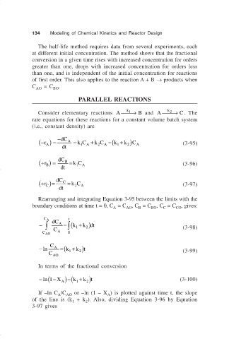
Consider elementary reactions A → B and A → C . The
k 1
k 2
rate equations for these reactions for a constant volume batch system
(i.e., constant density) are
k
− ( r A ) = −dC A = kC A + k C A =(k 1 + )C A (3-95)
2
1
2
dt
+ ( r B ) = dC B = kC A (3-96)
1
dt
+ ( r C )= dC C = kC A (3-97)
2
dt
Rearranging and integrating Equation 3-95 between the limits with the
boundary conditions at time t = 0, C = C , C = C , C = C , gives:
A AO B BO C CO

C A t
∫
− ∫ dC A = (k 1 + )dt
k
2
C A (3-98)
C AO 0
C
k
−ln A =(k 1 + )t (3-99)
2
C
AO
In terms of the fractional conversion
−
k
− (1 X A )=( 1 + )t (3-100)
ln
k
2
If –ln C /C AO or –ln (1 – X ) is plotted against time t, the slope
A
A
of the line is (k + k ). Also, dividing Equation 3-96 by Equation
1
2
3-97 gives