Page 132 - Modern Analytical Chemistry

1400-CH05 9/8/99 3:59 PM Page 115

Chapter 5 Calibrations, Standardizations, and Blank Corrections 115

–1
S spike = 0.266 + 312 mL ´V s
2+
Determine the concentration of Pb in the original sample of blood.
SOLUTION
To find the x-intercept we let S spike equal 0

–1
0 = 0.266 + 312 mL ´(x-intercept)
–4
and solve for the x-intercept’s absolute value, giving a value of 8.526 ´10 mL.
Thus
(.
CV C ´ 100 mL )
Ao
A
4 –
.
x-intercept = 8 526 ´10 mL = =
C S 1560 ppb
2+
and the concentration of Pb in the blood sample, C A , is 1.33 ppb.
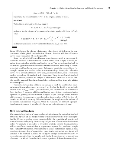
Figure 5.7(b) shows the relevant relationships when S spike is plotted versus the con-
centrations of the spiked standards after dilution. Standard addition calibration
curves based on equation 5.8 are also possible.
Since a standard additions calibration curve is constructed in the sample, it
cannot be extended to the analysis of another sample. Each sample, therefore, re-
quires its own standard additions calibration curve. This is a serious drawback to
the routine application of the method of standard additions, particularly in labora-
tories that must handle many samples or that require a quick turnaround time. For
example, suppose you need to analyze ten samples using a three-point calibration
curve. For a normal calibration curve using external standards, only 13 solutions
need to be analyzed (3 standards and 10 samples). Using the method of standard
additions, however, requires the analysis of 30 solutions, since each of the 10 sam-
ples must be analyzed three times (once before spiking and two times after adding
successive spikes).
The method of standard additions can be used to check the validity of an exter-
nal standardization when matrix matching is not feasible. To do this, a normal cali-
bration curve of S stand versus C S is constructed, and the value of k is determined
from its slope. A standard additions calibration curve is then constructed using
equation 5.6, plotting the data as shown in Figure 5.7(b). The slope of this standard
additions calibration curve gives an independent determination of k. If the two val-
ues of k are identical, then any difference between the sample’s matrix and that of
the external standards can be ignored. When the values of k are different, a propor-
tional determinate error is introduced if the normal calibration curve is used.

5 5 Internal Standards
B.
The successful application of an external standardization or the method of standard
additions, depends on the analyst’s ability to handle samples and standards repro-
ducibly. When a procedure cannot be controlled to the extent that all samples and
standards are treated equally, the accuracy and precision of the standardization may
suffer. For example, if an analyte is present in a volatile solvent, its concentration
will increase if some solvent is lost to evaporation. Suppose that you have a sample
and a standard with identical concentrations of analyte and identical signals. If both
experience the same loss of solvent their concentrations of analyte and signals will
continue to be identical. In effect, we can ignore changes in concentration due to
evaporation provided that the samples and standards experience an equivalent loss
of solvent. If an identical standard and sample experience different losses of solvent,