Page 135 - Modern Analytical Chemistry

1400-CH05 9/8/99 3:59 PM Page 118

118 Modern Analytical Chemistry

5
Table .2 Effect of a Constant Determinate Error on the Value
of k Calculated Using a Single-Point Standardization

C A S meas k S meas k
(true) (true) (with constant error) (apparent)
1.00 1.00 1.00 1.50 1.50
2.00 2.00 1.00 2.50 1.25
3.00 3.00 1.00 3.50 1.17
4.00 4.00 1.00 4.50 1.13
5.00 5.00 1.00 5.50 1.10
mean k(true) = 1.00 mean k (apparent) = 1.23

80 Table 5.2 demonstrates how an uncorrected constant error
affects our determination of k. The first three columns show
the concentration of analyte, the true measured signal (no
constant error) and the true value of k for five standards. As
60
expected, the value of k is the same for each standard. In the
fourth column a constant determinate error of +0.50 has
S meas 40 been added to the measured signals. The corresponding val-
ues of k are shown in the last column. Note that a different
value of k is obtained for each standard and that all values are
greater than the true value. As we noted in Section 5B.2, this
20
is a significant limitation to any single-point standardization.
How do we find the best estimate for the relationship be-
tween the measured signal and the concentration of analyte in
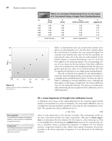
0 a multiple-point standardization? Figure 5.8 shows the data in
0.0 0.1 0.2 0.3 0.4 0.5 0.6
Table 5.1 plotted as a normal calibration curve. Although the
C A
data appear to fall along a straight line, the actual calibration
Figure 5.8 curve is not intuitively obvious. The process of mathemati-
Normal calibration plot of hypothetical data cally determining the best equation for the calibration curve is
from Table 5.1.
called regression.

5 C.1 Linear Regression of Straight-Line Calibration Curves
A calibration curve shows us the relationship between the measured signal and the
analyte’s concentration in a series of standards. The most useful calibration curve is
a straight line since the method’s sensitivity is the same for all concentrations of an-
alyte. The equation for a linear calibration curve is
y = b 0 + b 1 x 5.12
linear regression where y is the signal and x is the amount of analyte. The constants b 0 and b 1 are
A mathematical technique for fitting an the true y-intercept and the true slope, respectively. The goal of linear regres-
equation, such as that for a straight line,
sion is to determine the best estimates for the slope, b 1 , and y-intercept, b 0 . This
to experimental data.
is accomplished by minimizing the residual error between the experimental val-
ues, y i , and those values, ˆ y i , predicted by equation 5.12 (Figure 5.9). For obvious
residual error
The difference between an experimental reasons, a regression analysis is also called a least-squares treatment. Several ap-
value and the value predicted by a proaches to the linear regression of equation 5.12 are discussed in the following
regression equation. sections.