Page 139 - Modern Analytical Chemistry

1400-CH05 9/8/99 3:59 PM Page 122

122 Modern Analytical Chemistry

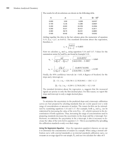
The results for all six solutions are shown in the following table.

x i y i ˆ y i (y i –ˆy i ) 2
0.000 0.00 0.209 0.0437
0.100 12.36 12.280 0.0064
0.200 24.83 24.350 0.2304
0.300 35.91 36.421 0.2611
0.400 48.79 48.491 0.0894
0.500 60.42 60.562 0.0202
Adding together the data in the last column gives the numerator of equation
5.15, S(y i – ˆ y i ) , as 0.6512. The standard deviation about the regression,
2
therefore, is
.
0 6512
.
s r = =0 4035
6 – 2
using equations 5.16 and 5.17. Values for the
Next we calculate s b1 and s b0
2
summation terms Sx and Sx i are found in Example 5.10.
i
2 2
6
ns r ()(. 0 4035 )
= = = . 0 965
s b 1 2 2 2
6
nx –( å x i ) ()(. 0 550 ) – ( . 1 500 )
å
i
2 2 2
0 4035) ( .
s å x i (. 0 550)
r
0 292
= = = .
s b 0 2 2 2
6 0 550) – ( .
n å x –( å x i ) ()(. 1 500)
i
Finally, the 95% confidence intervals (a= 0.05, 4 degrees of freedom) for the
slope and y-intercept are
= 120.706 ± (2.78)(0.965) = 120.7 ± 2.7
b 1 = b 1 ± ts b1
= 0.209 ± (2.78)(0.292) = 0.2 ± 0.8
b 0 = b 0 ± ts b0
The standard deviation about the regression, s r , suggests that the measured
signals are precise to only the first decimal place. For this reason, we report the
slope and intercept to only a single decimal place.
To minimize the uncertainty in the predicted slope and y-intercept, calibration
curves are best prepared by selecting standards that are evenly spaced over a wide
range of concentrations or amounts of analyte. The reason for this can be rational-
can be
ized by examining equations 5.16 and 5.17. For example, both s b0 and s b1
minimized by increasing the value of the term S(x i – x) , which is present in the de-
– 2
nominators of both equations. Thus, increasing the range of concentrations used in
preparing standards decreases the uncertainty in the slope and the y-intercept. Fur-
thermore, to minimize the uncertainty in the y-intercept, it also is necessary to de-
2
crease the value of the term Sx in equation 5.17. This is accomplished by spreading
i
the calibration standards evenly over their range.
Using the Regression Equation Once the regression equation is known, we can use
it to determine the concentration of analyte in a sample. When using a normal cali-
bration curve with external standards or an internal standards calibration curve, we
–
measure an average signal for our sample, Y X, and use it to calculate the value of X