Page 143 - Modern Analytical Chemistry

1400-CH05 9/8/99 3:59 PM Page 126

126 Modern Analytical Chemistry

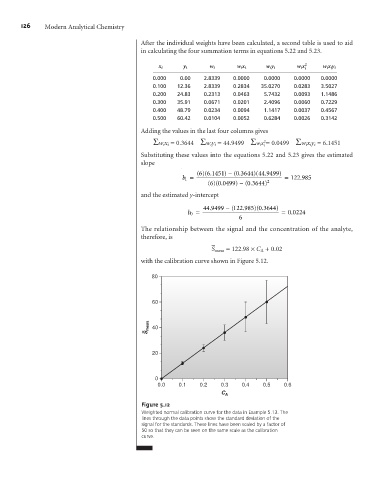
After the individual weights have been calculated, a second table is used to aid
in calculating the four summation terms in equations 5.22 and 5.23.

x i y i w i w i x i w i y i w i x 2 i w i x i y i
0.000 0.00 2.8339 0.0000 0.0000 0.0000 0.0000
0.100 12.36 2.8339 0.2834 35.0270 0.0283 3.5027
0.200 24.83 0.2313 0.0463 5.7432 0.0093 1.1486
0.300 35.91 0.0671 0.0201 2.4096 0.0060 0.7229
0.400 48.79 0.0234 0.0094 1.1417 0.0037 0.4567
0.500 60.42 0.0104 0.0052 0.6284 0.0026 0.3142
Adding the values in the last four columns gives
2
Sw ix i = 0.3644 Sw iy i = 44.9499 Sw i x = 0.0499 Sw ix iy i = 6.1451
i
Substituting these values into the equations 5.22 and 5.23 gives the estimated
slope
()(. 0 3644 44 9499)
)( .
6 6 1451) – (.
.
b 1 = = 122 985
()(. 0 3644) 2
6 0 0499) – (.
and the estimated y-intercept
.
44 9499 – ( 122 985 0 3644)
.
.
(
)
.
b 0 = = 0 0224
6
The relationship between the signal and the concentration of the analyte,
therefore, is
–
S meas = 122.98 ´C A + 0.02
with the calibration curve shown in Figure 5.12.
80
60

S meas 40

20

0
0.0 0.1 0.2 0.3 0.4 0.5 0.6
C A
Figure 5.12
Weighted normal calibration curve for the data in Example 5.13. The
lines through the data points show the standard deviation of the
signal for the standards. These lines have been scaled by a factor of
50 so that they can be seen on the same scale as the calibration
curve.