Page 140 - Modern Analytical Chemistry

1400-CH05 9/8/99 3:59 PM Page 123

Chapter 5 Calibrations, Standardizations, and Blank Corrections 123

Y X – b 0
X =
b 1 5.20
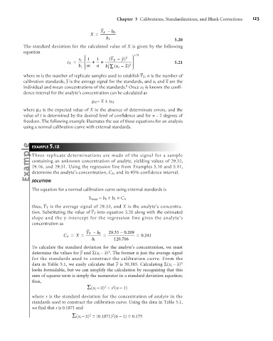
The standard deviation for the calculated value of X is given by the following
equation
12 /
ì
s ï1 1 ( Y X – y) 2 ü
ï
r
s X = í + + ý 5.21
2
2
)
b ï m n b å( x – x ï
i
1
1
î þ
–
where m is the number of replicate samples used to establish Y X , n is the number of
–
–
calibration standards, y is the average signal for the standards, and x i and x are the
8
individual and mean concentrations of the standards. Once s X is known the confi-
dence interval for the analyte’s concentration can be calculated as
m X = X ± ts X
where m X is the expected value of X in the absence of determinate errors, and the
value of t is determined by the desired level of confidence and for n – 2 degrees of
freedom. The following example illustrates the use of these equations for an analysis
using a normal calibration curve with external standards.
EXAMPLE 5 .12
Three replicate determinations are made of the signal for a sample
containing an unknown concentration of analyte, yielding values of 29.32,
29.16, and 29.51. Using the regression line from Examples 5.10 and 5.11,
determine the analyte’s concentration, C A , and its 95% confidence interval.
SOLUTION

The equation for a normal calibration curve using external standards is
S meas = b 0 + b 1 ´C A
–
thus, Y X is the average signal of 29.33, and X is the analyte’s concentra-
–
tion. Substituting the value of Y X into equation 5.20 along with the estimated
slope and the y-intercept for the regression line gives the analyte’s
concentration as

.
.
29 33 – 0 209
Y– b 0
X
.
C A = X = = =0 241
.
b 1 120 706
To calculate the standard deviation for the analyte’s concentration, we must
–
determine the values for y and S(x i – x) . The former is just the average signal
– 2
for the standards used to construct the calibration curve. From the
–
data in Table 5.1, we easily calculate that y is 30.385. Calculating S(x i – x)
– 2
looks formidable, but we can simplify the calculation by recognizing that this
sum of squares term is simply the numerator in a standard deviation equation;
thus,
– 2
S(x i – x) = s (n –1)
2
where s is the standard deviation for the concentration of analyte in the
standards used to construct the calibration curve. Using the data in Table 5.1,
we find that s is 0.1871 and
2
– 2
S(x i – x) = (0.1871) (6 – 1) = 0.175