Page 141 - Modern Analytical Chemistry

1400-CH05 9/8/99 3:59 PM Page 124

124 Modern Analytical Chemistry

Substituting known values into equation 5.21 gives
12 /
0 4035 ì 1 1 (. 30 385) 2 ü
.
.
29 33 –
s A = s X = í + + ý = 0 0024.
2
.
.
.
120 706 ï 3 6 ( 120 706) ( 0 175) ï
î þ
Finally, the 95% confidence interval for 4 degrees of freedom is
m A = C A ± ts A = 0.241 ±(2.78)(0.0024) = 0.241 ± 0.007
In a standard addition the analyte’s concentration is determined by extrapolat-
ing the calibration curve to find the x-intercept. In this case the value of X is
b – 0
X = x-intercept =
b 1
and the standard deviation in X is
Residual error 0 s X = s ï 1 + b å ( x – x) 2 ü 12 /
ì
2
y ( )
ï
r
ý
í
2
n
b ï
ï
1
i
þ
1
î

where n is the number of standards used in preparing the standard additions cali-
–
bration curve (including the sample with no added standard), and y is the average
x i signal for the n standards. Because the analyte’s concentration is determined by ex-
(a) trapolation, rather than by interpolation, s X for the method of standard additions
generally is larger than for a normal calibration curve.
A linear regression analysis should not be accepted without evaluating the
validity of the model on which the calculations were based. Perhaps the simplest
Residual error 0 for each value of x. The residual error for a single calibration standard, r i , is given as
way to evaluate a regression analysis is to calculate and plot the residual error
r i = y i – ˆ y i
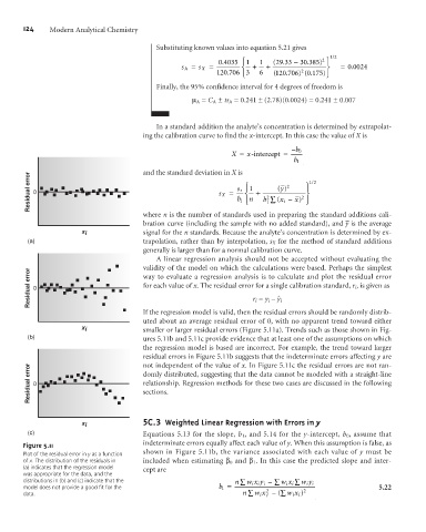
If the regression model is valid, then the residual errors should be randomly distrib-
uted about an average residual error of 0, with no apparent trend toward either
x i smaller or larger residual errors (Figure 5.11a). Trends such as those shown in Fig-
(b) ures 5.11b and 5.11c provide evidence that at least one of the assumptions on which
the regression model is based are incorrect. For example, the trend toward larger
residual errors in Figure 5.11b suggests that the indeterminate errors affecting y are
not independent of the value of x. In Figure 5.11c the residual errors are not ran-
Residual error 0 domly distributed, suggesting that the data cannot be modeled with a straight-line
relationship. Regression methods for these two cases are discussed in the following
sections.
5 3
x i C. Weighted Linear Regression with Errors in y
(c) Equations 5.13 for the slope, b 1 , and 5.14 for the y-intercept, b 0 , assume that
Figure 5.11 indeterminate errors equally affect each value of y. When this assumption is false, as
shown in Figure 5.11b, the variance associated with each value of y must be
Plot of the residual error in y as a function
of x. The distribution of the residuals in included when estimating b 0 and b 1 . In this case the predicted slope and inter-
(a) indicates that the regression model cept are
was appropriate for the data, and the
distributions in (b) and (c) indicate that the n å w xy i – å wx å wy i
ii
ii
i
model does not provide a good fit for the b 1 = 2 2 5.22
data. n å w x –( å w x )
i
ii
i