Page 142 - Modern Analytical Chemistry

1400-CH05 9/8/99 3:59 PM Page 125

Chapter 5 Calibrations, Standardizations, and Blank Corrections 125

and
å wy – b 1å w x i
ii
i
b 0 = 5.23
n
where w i is a weighting factor accounting for the variance in measuring y i . Values of
w i are calculated using equation 5.24.
ns –2
i
w i = 5.24
å s –2
i
where s i is the standard deviation associated with y i . The use of a weighting factor
ensures that the contribution of each pair of xy values to the regression line is pro-
portional to the precision with which y i is measured.

5 3
EXAMPLE .1
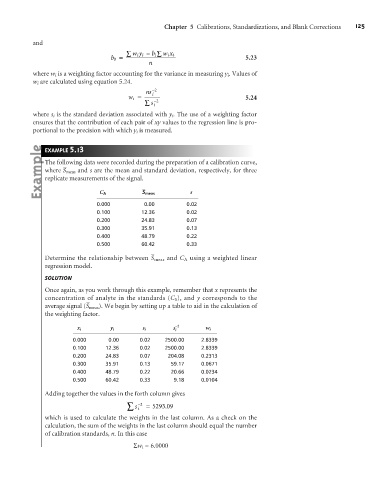
The following data were recorded during the preparation of a calibration curve,
–
where S meas and s are the mean and standard deviation, respectively, for three
replicate measurements of the signal.
–
C A S meas s
0.000 0.00 0.02
0.100 12.36 0.02
0.200 24.83 0.07
0.300 35.91 0.13
0.400 48.79 0.22
0.500 60.42 0.33
–
Determine the relationship between S meas and C A using a weighted linear
regression model.

SOLUTION
Once again, as you work through this example, remember that x represents the
concentration of analyte in the standards (C S ), and y corresponds to the
–
average signal (S meas). We begin by setting up a table to aid in the calculation of
the weighting factor.

x i y i s i s –2 w i
i
0.000 0.00 0.02 2500.00 2.8339
0.100 12.36 0.02 2500.00 2.8339
0.200 24.83 0.07 204.08 0.2313
0.300 35.91 0.13 59.17 0.0671
0.400 48.79 0.22 20.66 0.0234
0.500 60.42 0.33 9.18 0.0104
Adding together the values in the forth column gives

å s –2 = 5293 .09
i
which is used to calculate the weights in the last column. As a check on the
calculation, the sum of the weights in the last column should equal the number
of calibration standards, n. In this case
Sw i = 6.0000