Page 137 - Modern Analytical Chemistry

1400-CH05 9/8/99 3:59 PM Page 120

120 Modern Analytical Chemistry

x 2
x i y i x i y i
i
0.000 0.00 0.000 0.000
0.100 12.36 0.010 1.236
0.200 24.83 0.040 4.966
0.300 35.91 0.090 10.773
0.400 48.79 0.160 19.516
0.500 60.42 0.250 30.210
Adding the values in each column gives
2
Sx i = 1.500 Sy i = 182.31 Sx i = 0.550 Sx iy i = 66.701
Substituting these values into equations 5.12 and 5.13 gives the estimated slope
()( . 1 500 182 31)
.
)(
6 66 701) – ( .
b 1 = 2 = 120 706
.
6 0 550) – ( .
()(. 1 500)
and the estimated y-intercept
.
)
182 31 – ( 120 706 1 500)
.
.
(
b 0 = = 0 209
.
6
The relationship between the signal and the analyte, therefore, is
S meas = 120.70 ´C S + 0.21
Note that for now we keep enough significant figures to match the number of
decimal places to which the signal was measured. The resulting calibration
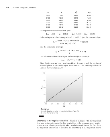
curve is shown in Figure 5.10.
80

60

S meas 40

20

0
0.0 0.1 0.2 0.3 0.4 0.5 0.6
C A
Figure 5.10
Normal calibration curve for the hypothetical data in Table 5.1,
showing the regression line.

Uncertainty in the Regression Analysis As shown in Figure 5.10, the regression
line need not pass through the data points (this is the consequence of indeter-
minate errors affecting the signal). The cumulative deviation of the data from
the regression line is used to calculate the uncertainty in the regression due to