
Page 136 - Modern Analytical Chemistry
P. 136
1400-CH05 9/8/99 3:59 PM Page 119
Chapter 5 Calibrations, Standardizations, and Blank Corrections 119
5C.2 Unweighted Linear Regression with Errors in y Regression
line
The most commonly used form of linear regression is based on three assump-
tions: (1) that any difference between the experimental data and the calculated
regression line is due to indeterminate errors affecting the values of y, (2) that
these indeterminate errors are normally distributed, and (3) that the indetermi-
nate errors in y do not depend on the value of x. Because we assume that indeter-
minate errors are the same for all standards, each standard contributes equally in
ˆ y i
estimating the slope and y-intercept. For this reason the result is considered an
unweighted linear regression.
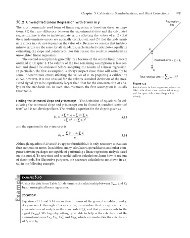
The second assumption is generally true because of the central limit theorem Residual error = y – ˆy
outlined in Chapter 4. The validity of the two remaining assumptions is less cer- i i
tain and should be evaluated before accepting the results of a linear regression.
In particular, the first assumption is always suspect since there will certainly be y i
some indeterminate errors affecting the values of x. In preparing a calibration 2
Total residual error = ∑ (y – ˆy )
i
i
curve, however, it is not unusual for the relative standard deviation of the mea-
sured signal (y) to be significantly larger than that for the concentration of ana- Figure 5.9
lyte in the standards (x). In such circumstances, the first assumption is usually Residual error in linear regression, where the
reasonable. filled circle shows the experimental value y i ,
and the open circle shows the predicted
value ˆ y i .
Finding the Estimated Slope and y-Intercept The derivation of equations for cal-
culating the estimated slope and y-intercept can be found in standard statistical
7
texts and is not developed here. The resulting equation for the slope is given as
n å x y – å x i å y i
ii
b 1 = 2 2 5.13
n å x –( å x i )
i
and the equation for the y-intercept is
å y i – b 1 å x i
b 0 = 5.14
n
Although equations 5.13 and 5.14 appear formidable, it is only necessary to evaluate
four summation terms. In addition, many calculators, spreadsheets, and other com-
puter software packages are capable of performing a linear regression analysis based
on this model. To save time and to avoid tedious calculations, learn how to use one
of these tools. For illustrative purposes, the necessary calculations are shown in de-
tail in the following example.
5
EXAMPLE .10
Using the data from Table 5.1, determine the relationship between S meas and C S
by an unweighted linear regression.
SOLUTION
Equations 5.13 and 5.14 are written in terms of the general variables x and y.
As you work through this example, remember that x represents the
concentration of analyte in the standards (C S ), and that y corresponds to the
signal (S meas ). We begin by setting up a table to help in the calculation of the
2
summation terms Sx i , Sy i , Sx i , and Sx i y i which are needed for the calculation
of b 0 and b 1