Page 245 - Modern Control Systems

Exercises 219

E3.15 Consider the case of the two masses connected as where R, L u L 2 and C are given constants, and -¾ and
shown in Figure E3.15. The sliding friction of each v h are inputs. Let the state variables be defined as
mass has the constant b. Determine a state variable *! = I'I, x 2 = l 2, and x 3 = v. Obtain a state variable
matrix differential equation. representation of the system where the output is x 3.
E3.19 A single-input, single-output system has the matrix
equations

and
y = [10 0]x.
Determine the transfer function G(s) = Y(s)/U(s).
FIGURE E3.15 Two-mass system. Answer: G(s) = -z 1°
s + 4s + 3
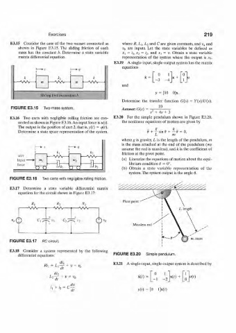
E3.16 Two carts with negligible rolling friction are con- E3.20 For the simple pendulum shown in Figure E3.20,
nected as shown in Figure E3.16. An input force is u(t). the nonlinear equations of motion are given by
The output is the position of cart 2. that is, y{t) = q(t).
Determine a state space representation of the system. e + f- sin e + —e = o,
L m
where g is gravity, L is the length of the pendulum, m
is the mass attached at the end of the pendulum (we
assume the rod is massless), and k is the coefficient of
friction at the pivot point.
H(0
Inpul ' m 2 (a) Linearize the equations of motion about the equi-
force Hi Hi librium condition 6 = 0",
(b) Obtain a state variable representation of the
system. The system output is the angle 6.
FIGURE E3.16 Two carts with negligible rolling friction.

E3.17 Determine a state variable differential matrix ZZ&ZZZX&&
equation for the circuit shown in Figure E3.17:

Pivot point

Massless rod

FIGURE E3.17 RC circuit. in, mass
E3.18 Consider a system represented by the following
FIGURE E3.20 Simple pendulum.
differential equations:
rf/, E3.21 A single-input, single-output system is described by
R>i + L t — + v = v„
di 2 0 I
L + V = V x(r) = X(f) + M(0
^ " -1 0
dv
= C
i x + i 2
~dt v(0 = [o i]x«