Page 249 - Modern Control Systems

Problems 223
of the depth of a submarine. The equations describing Elbow ^i
the dynamics of a submarine can be obtained by using Wrist
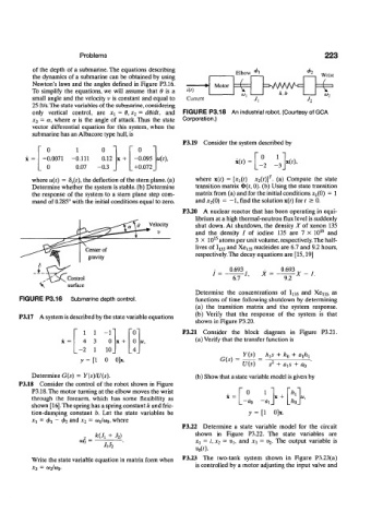
Newton's laws and the angles defined in Figure P3.16. Motor 4= VvWA k
To simplify the equations, we will assume that 8 is a Kr) k,b
small angle and the velocity v is constant and equal to Current h
25 ft/s.The state variables of the submarine, considering
only vertical control, are X\ = 6, x 2 = dOldt, and FIGURE P3.18 An industrial robot. (Courtesy of GCA
x$ = a, where a is the angle of attack. Thus the state Corporation.)
vector differential equation for this system, when the
submarine has an Albacore type hull, is
P3.19 Consider the system described by
0 1 0 0
x = 0.0071 -0.111 0.12 x + -0.095 u(t\ i(0 = 0 1 x(0«
0 0.07 -0.3 +0.072 - 2
T
where u{t) = 8 s(t), the deflection of the stem plane, (a) where x(t) = [* a(/) x 2(t)] . (a) Compute the state
Determine whether the system is stable, (b) Determine transition matrix $(f, 0). (b) Using the state transition
the response of the system to a stern plane step com- matrix from (a) and for the initial conditions JC^O) = 1
-
mand of 0.285° with the initial conditions equal to zero. and x 2(0) = 1 , find the solution x(r) for t > 0.
P3.20 A nuclear reactor that has been operating in equi-
librium at a high thermal-neutron flux level is suddenly
0 Velocity shut down. At shutdown, the density X of xenon 135
v and the density I of iodine 135 are 7 X 10 16 and
15
3 X 10 atoms per unit volume, respectively. The half-
lives of I 135 and Xej35 nucleides are 6.7 and 9.2 hours,
respectively. The decay equations are [15,19]

0.693 0.693
I = 1, X = X - I.
„ -\^J\ Control ' 6.7 " 9.2
\ . surface
Determine the concentrations of I 135 and Xei 35 as
FIGURE P3.16 Submarine depth control. functions of time following shutdown by determining
(a) the transition matrix and the system response.
(b) Verify that the response of the system is that
P3.17 A system is described by the state variable equations
shown in Figure P3.20.
1 1 - 1 0 P3.21 Consider the block diagram in Figure P3.21.
4 3 0 x + 0 (a) Verify that the transfer function is
-2 1 10_ _4
Y(s) h xs + h 0 + a xh x
y = [l 0 0]x. G(s) = z
U(s) s + ais + a 0
Determine G(s) = Y(s)/U(s). (b) Show that a state variable model is given by
P3.18 Consider the control of the robot shown in Figure
P3.18.The motor turning at the elbow moves the wrist 0 1
through the forearm, which has some flexibility as x + u,
shown [16]. The spring has a spring constant k and fric-
tion-damping constant b. Let the state variables be y = [l 0]x.
*i = 4>\ ~ $2 and x 2 = (O^COQ, where
P3.22 Determine a state variable model for the circuit
shown in Figure P3.22. The state variables are
a>l = JCJ = I, x 2 = V\, and x 3 = 1¾. The output variable is

Write the state variable equation in matrix form when P3.23 The two-tank system shown in Figure P3.23(a)
x 3 = a) 2Ia> 0. is controlled by a motor adjusting the input valve and