Page 248 - Modern Control Systems

222 Chapter 3 State Variable Models

= 0.5. (a) Determine the closed-loop transfer
K y (a) Determine a state variable model.
function (b) Determine $(0, the state transition matrix.
Tis) (o(s) P3.13 Consider again the RLC circuit of Problem
= m P3.1 when R = 2.5, L = 1/4. and C = 1/6. (a) De-
(b) Determine a state variable representation, (c) De- termine whether the system is stable by finding the
termine the characteristic equation obtained from the characteristic equation with the aid of the A ma-
A matrix. trix. (b) Determine the transition matrix of the
network, (c) When the initial inductor current is 0.1
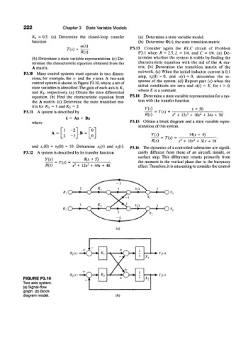
P3.10 Many control systems must operate in two dimen- amp, v c(0) = 0, and v(t) = 0, determine the re-
sions, for example, the x- and the y-axes. A two-axis sponse of the system, (d) Repeat part (c) when the
control system is shown in Figure P3.10, where a set of initial conditions are zero and v(t) = E, for t > 0,
state variables is identified.The gain of each axis is Ki where E is a constant.
and K 2, respectively, (a) Obtain the state differential
equation, (b) Find the characteristic equation from P3.14 Determine a state variable representation for a sys-
the A matrix, (c) Determine the state transition ma- tem with the transfer function
trix for Ki = 1 and K 2 = 2.
s + 50
P3.ll A system is described by = T(s) = A 3 2
R(s) s + 12s + IO5 + 34s + 50'
x = Ax + Bu
where P3.15 Obtain a block diagram and a state variable repre-
sentation of this system.
1 -2~ V
A = 2 ,B = u y(s) U(s + 4)
L -3 J L J = =
R(s) ^ s 3 + io.v 2 + 31s + 16'
and X](0) = x 2(0) = 10. Determine x {(t) and x 2(t). P3.16 The dynamics of a controlled submarine are signifi-
P3.12 A system is described by its transfer function cantly different from those of an aircraft, missile, or
surface ship. This difference results primarily from
Y(s) _ 8(5 + 5)
T(s) = the moment in the vertical plane due to the buoyancy
R~(s) effect. Therefore, it is interesting to consider the control

R.O—+ +—Or,

K2O "*—0 2

(a)

• y,(s)

1—*- >Uv)
FIGURE P3.10
Two-axis system.
(a) Signal-flow
graph, (b) Block
diagram model. (b)