Page 258 - Modern Control Systems

232 Chapter 3 State Variable Models

and CP3.7 Consider the following system:
0.5000 0.5000 0.7071 0 0 1 x +
0.5000 -0.5000 0.7071 x 2 + 0 L-2 -3 J
6.3640 -0.7071 - 8.000 _ 4 y = [l 0]x
= [0.7071 -0.7071 0]x 2. ( (2) with
(a) Using the tf function, determine the transfer func- x(0)
tion Y(s)/U(s) for system (1).
(b) Repeat part (a) for system (2). Using the Isim function obtain and plot the system
(c) Compare the results in parts (a) and (b) and response (for x x(t) and JC 2(/)) when u(t) = 0.
comment.
CP3.8 Consider the state variable model with parameter
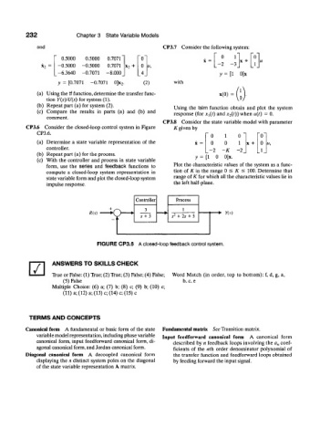
CP3.6 Consider the closed-loop control system in Figure K given by
CP3.6.
~ o l o 1 To"
(a) Determine a state variable representation of the 0 0 1 x + 0 M,
controller. . - 2 -K -2 J L .
1
(b) Repeat part (a) for the process.
(c) With the controller and process in state variable i o o]x.
form, use the series and feedback functions to Plot the characteristic values of the system as a func-
compute a closed-loop system representation in tion of K in the range 0 ^ K < 100. Determine that
state variable form and plot the closed-loop system range of K for which all the characteristic values he in
impulse response. the left half-plane.

Controller Process
3 I
— • 2 ** Y(s)
5 + 3 s + 2s + 5
i.

FIGURE CP3.6 A closed-loop feedback control system.

ANSWERS TO SKILLS CHECK

m True or False: (1) True; (2) True; (3) False; (4) False; Word Match (in order, top to bottom): f, d, g, a,
(5) False b, c, e
Multiple Choice: (6) a; (7) b; (8) c; (9) b; (10) c;
(11) a; (12) a; (13) c; (14) c; (15) c

TERMS AND CONCEPTS
Canonical form A fundamental or basic form of the state Fundamental matrix See Transition matrix.
variable model representation, including phase variable Input feedforward canonical form A canonical form
canonical form, input feedforward canonical form, di- described by n feedback loops involving the a n coef-
agonal canonical form, and Jordan canonical form. ficients of the nth order denominator polynomial of
Diagonal canonical form A decoupled canonical form the transfer function and feedforward loops obtained
displaying the n distinct system poles on the diagonal by feeding forward the input signal.
of the state variable representation A matrix.