
Page 295 - Modern Control Systems
P. 295
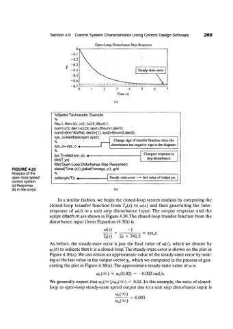
Section 4.9  Control System  Characteristics  Using Control  Design Software  2 6 9
                                           Open-Loop Disturbance Step Response
                                   0
                                 -0.1
                                 -0.2  V                        j
                                 -0.3
                                 -0.4    \                    Steady-state error
                                 -0.5
                                 -0.6       ^ ^ - - _ _ _             \
                                 -0.7
                                    0     1  2       3    4     5     6    7
                                                     Time (s)
                                                    (a)


                         %Speed Tachometer  Example
                         %
                         Ra=1; Km=10; J=2; f=0.5; Kb=0.1;
                         num1=[1]; den1=[J,b]; sys1=tf(num1,den1);
                         num2=[Km*Kb/Ra]; den2=[1]; sys2=tf(num2,den2);
                         sys_o=feedback(sys1 ,sys2);
                                                    Change sign of transfer function  since the
                         %
                                                   disturbance has negative sign in the diagram.
                         sys_o=-sys_o •*
                         %
                         [yo,T]=step(sys_o); ^                   Compute response to
                                                                  step disturbance.
                         plot{T,yo)
                         title('Open-Loop  Disturbance Slep  Response')
       FIGURE  4.29      xlabel(Time (s)'),ylabel('\omega_o'), grid
      Analysis of the    %
       open-loop speed   yo(length(T))  4         Steady-state error —•  last value of output yo.
       control system.
       (a) Response.
       (b) m-file script.                           (b)
                           In a similar fashion, we begin the closed-loop system analysis by computing the
                       closed-loop  transfer  function  from  T (i(s) to  (o(s)  and  then  generating  the  time-
                       response  of  (o(t)  to  a unit  step  disturbance  input. The  output  response  and  the
                       script  cltach.m are shown in Figure 4.30. The closed-loop transfer  function  from  the
                       disturbance input  (from  Equation  (4.30)) is
                                                          - 1
                                               T d(s)  2s  +  541.5  sys_c.
                       As before, the  steady-state  error  is just  the  final  value  of  <o(t),  which  we denote  by
                       w c(t) to indicate that it is a closed-loop. The steady-state error is shown on the plot in
                       Figure 4.30(a). We can obtain an approximate value of the steady-state error by look-
                       ing at the last value in the output vector y c, which we computed in the process of gen-
                       erating the plot in Figure 4.30(a). The approximate steady-state value  of <o is
                                            w c(oo)  «  <u f (0.02)  =  -0.002 rad/s.

                       We generally expect that <o c(oo)/a) 0(oo)  <  0.02. In this example, the ratio of closed-
                       loop to open-loop steady-state  speed  output  due to a unit step disturbance  input is
                                                    (o c{oo)
                                                           =  0.003.
                                                    <*o{ OO)