Page 297 - Modern Control Systems

Section 4.9 Control System Characteristics Using Control Design Software 271
Step Response for K= 100
1.5
•
•
1.0
a
Overshoot
0.5 Settling time
i , |
0
0 0.2 0.4 0.6 0.8 1.0 1.2 1.4 1.6 1.8 2.0
Time (s)
(a)

Step Response tor K =20

1.0 i
/ - > i i
0.5 j Overshoot Settling time

\
0 0.2 0.4 0.6 0.8 1.0 1.2 1. 1.6 1.8 2.0
Time (s)
(b)

% Response to a Unit Step Input R(s)=1/s for K=20 and K=100
%
numg=[1]; deng=[1 1 0]; sysg=tf(numg,deng);
K1=100;K2=20;
num1=[11 K1]; num2=[11 K2]; den=[0 1];
sys1=tf(num1,den);
sys2=tf(num2,den);
%
sysa=series(sys1 ,sysg); sysb=series(sys2,sysg); Closed-loop
sysc=feedback(sysa,[1]); sysd=feedback(sysb,[1]); transfer functions.
/o
t=[0:0.01:2.0]; < Choose time interval.
[y1 ,t]=slep(sysc,t); [y2,t]=step(sysd,t);
subplot(211),plot(t,y1), title('Step Response for K=100') Create subplots
,
FIGURE 4.31 xlabel('Time (s)'),ylabel( y(t)'), grid -4 with x and y
The response to a subplot(212),plot(t,y2), title('Step Response for K=20') axis labels.
step input when xlabel(Time (sJ'J.ylabelCy^)'), grid
(a)K= 100 and
(b) K = 20.
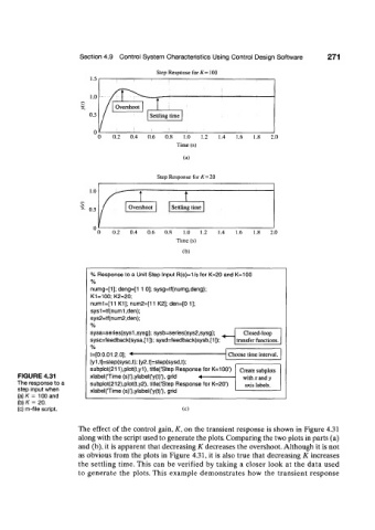
(c) m-file script. (c)

The effect of the control gain, K, on the transient response is shown in Figure 4.31
along with the script used to generate the plots. Comparing the two plots in parts (a)
and (b), it is apparent that decreasing K decreases the overshoot. Although it is not
as obvious from the plots in Figure 4.31, it is also true that decreasing K increases
the settling time. This can be verified by taking a closer look at the data used
to generate the plots. This example demonstrates how the transient response