Page 300 - Modern Control Systems

274 Chapter 4 Feedback Control System Characteristics

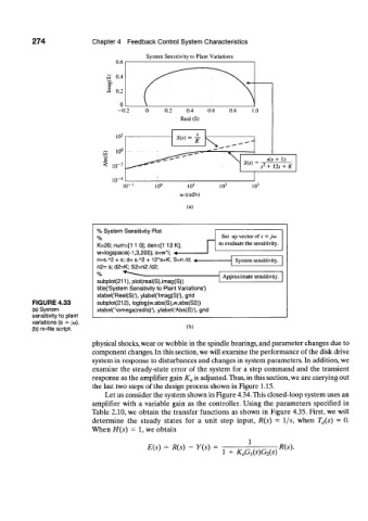
System Sensitivity to Plant Variations

0.2 0.4 0.6 0.8
Real (S)

(a)

% System Sensitivity Plot
% Set up vector of s = jco
K=20; num=[1 1 0]; den=[1 12 K]; to evaluate the sensitivity.
w=logspace(-1,3,200); s=w*i; •«—
A
A
n=s. 2 + s; d= s. 2 + 12*s+K; S=n./d; ««- System sensitivity.
n2= s; d2=K; S2=n2./d2;
Approximate sensitivity.
subplot(211), plot(real(S),imag(S))
title('System Sensitivity to Plant Variations')
xlabel('Real(S)'), ylabel('lmag(S)') ) grid
FIGURE 4.33 subplot(212), loglog(w,abs(S),w,abs(S2))
(a) System xlabel('\omega(rad/s)'), ylabel('Abs(S)'), grid
sensitivity to plant
variations (s = jw).
(b) m-file script. (b)
physical shocks, wear or wobble in the spindle bearings, and parameter changes due to
component changes. In this section, we will examine the performance of the disk drive
system in response to disturbances and changes in system parameters. In addition, we
examine the steady-state error of the system for a step command and the transient
response as the amplifier gain K a is adjusted. Thus, in this section, we are carrying out
the last two steps of the design process shown in Figure 1.15.
Let us consider the system shown in Figure 4.34.This closed-loop system uses an
amplifier with a variable gain as the controller. Using the parameters specified in
Table 2.10, we obtain the transfer functions as shown in Figure 4.35. First, we will
determine the steady states for a unit step input, R{s) = 1/s, when T (i(s) = 0.
When H(s) = 1, we obtain

1
E(s) = R(s) - Y(s) = R(s).
1 + K aG 1(s)G 2{s)