Page 296 - Modern Control Systems
P. 296

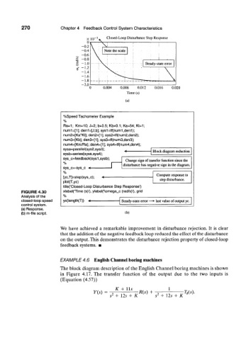
270              Chapter  4  Feedback  Control System  Characteristics

                                               Closed-Loop Disturbance  Step Response


                                                                Steady-state error


                                              0.004   0.008  0.012  0.016   0.020
                                                        Time (s)
                                                       (a)


                            %Speed Tachometer  Example
                            %
                            Ra=1;  Km=10; J=2; b=0.5; Kb=0.1; Ka=54; Kt=1;
                            num1=[1]; den1=[J,b]; sys1=tf{num1,den1);
                            num2=[Ka*Kt]; den2=[1]; sys2=tf(num2,den2);
                            num3=[Kb]; den3=[1]; sys3=tf(num3,den3);
                            num4=[Km/Ra]; den4=[1]; sys4=tf(num4,den4);
                            sysa=parallel(sys2,sys3);
                                                                   Block diagram reduction
                            sysb=series(sysa,sys4);
                            sys_c=feedback(sys1 ,sysb);   Change sign of transfer function  since the
                            %
                                                      disturbance has negative sign in the diagram.
                            sys_c=-sys_c  <
                            %
                                                                    Compute response to
                            [yc,T]=step(sys_c);  M
                                                                      step disturbance.
                            plot(T,yc)
                            tille('Closed-Loop  Disturbance Step  Response')
          FIGURE  4.30      xlabel(Time (s)'), ylabelC\omega_c (rad/s)'), grid
          Analysis of the   %
          closed-loop speed   yc(length(T))  *4      Steady-state error —•  last value of output yc.
          control system.
          (a) Response.
          (b) m-file script.                           (b)

                           We have  achieved  a  remarkable  improvement  in  disturbance  rejection.  It  is clear
                           that the addition  of the negative feedback  loop reduced the effect  of the disturbance
                           on the output. This demonstrates the  disturbance  rejection  property  of closed-loop
                           feedback  systems.  •


                           EXAMPLE   4.6  English Channel boring  machines
                           The block diagram description  of the English  Channel boring machines is shown
                           in  Figure  4.17. The  transfer  function  of  the  output  due  to  the  two  inputs  is
                           (Equation  (4.57))

                                                   K  +  Us              1
                                         Y(s)  =  2          R(s)  +  2         Us).
                                                s  +  12s + K       5  +  lZv  +  K
   291   292   293   294   295   296   297   298   299   300   301