Page 344 - Modern Control Systems

318 Chapter 5 The Performance of Feedback Control Systems

L, > 0.707
and

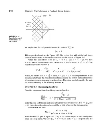
FIGURE 5.15
Specifications and
root locations on
the s-plane.

we require that the real part of the complex poles of T(s) be

fan ^ I-
This region is also shown in Figure 5.15. The region that will satisfy both time-
domain requirements is shown cross-hatched on the s-plane of Figure 5.15.
When the closed-loop roots are r\ = — 1 + /1 and ?\ = - 1 - ) 1 , we have
= 4 s and an overshoot of 4.3%. Therefore, £ = l / v 2 and co t, = l/£ = V 2. The
T s
closed-loop transfer function is
G(s) K 0)7,
T(s) 2 2
2'
1 + G(s) s + ps + K s + 2fa ns + (of,
2
Hence, we require that K = w , = 2 and p - 2£io„ = 2. A full comprehension of the
correlation between the closed-loop root location and the system transient response
is important to the system analyst and designer. Therefore, we shall consider the mat-
ter more completely in the following sections. •

EXAMPLE 5.2 Dominant poles of T(s)

Consider a system with a closed-loop transfer function

— (s + a)
Y{s)
= T{s) =
2
R(s) (s 2 + 2(a> Hs + <o „)(\ + rs)
Both the zero and the real pole may affect the transient response. If a » fan a n d
T « \/fa u, then the pole and zero will have little effect on the step response.
Assume that we have
62.5(4' + 2.5)
T(s) = 2
(,v + 6A- + 25)(s + 6.25)
Note that the DC gain is equal to 1 (T(0) = 1), and we expect a zero steady-state
error for a step input. We have £a>„ = 3, T = 0.16, and a = 2.5. The poles and the