Page 341 - Modern Control Systems

Section 5.4 Effects of a Third Pole and a Zero on the Second-Order System Response 315

je>

• = roots of the ,'
closed-loop /^s,
system / v. I

-<r

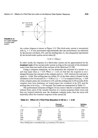
FIGURE 5.12 X
An s-plane diagram
of a third-order
system.

the s-plane diagram is shown in Figure 5.12. This third-order system is normalized
with co„ = 1. It was ascertained experimentally that the performance (as indicated
by the percent overshoot, P.O., and the settling time, 7^.), was adequately represented
by the second-order system curves when [4]
|l/y| > 10|faJ.

In other words, the response of a third-order system can be approximated by the
dominant roots of the second-order system as long as the real part of the dominant
roots is less than one tenth of the real part of the third root [15,20].
Using a computer simulation, we can determine the response of a system to a
unit step input when £ = 0.45. When y = 2.25, we find that the response is over-
damped because the real part of the complex poles is —0.45, whereas the real pole is
equal to -0.444. The settling time (to within 2% of the final value) is found via the
simulation to be 9.6 seconds. If y = 0.90 or l/y = 1.11 is compared with ga) n = 0.45
of the complex poles, the overshoot is 12% and the settling time is 8.8 seconds. If the
complex roots were dominant, we would expect the overshoot to be 20% and the
settling time to be 4/£w„ = 8.9 seconds. The results are summarized in Table 5.3.
The performance measures of Figure 5.8 are correct only for a transfer function
without finite zeros. If the transfer function of a system possesses finite zeros and
they are located relatively near the dominant complex poles, then the zeros will
materially affect the transient response of the system [5J.

Table 5.3 Effect of a Third Pole (Equation 5.18) for £ = 0.45
1
— Percent Settling
r 7 Overshoot Time*
2.25 0.444 0 9.63
1.5 0.666 3.9 6.3
0.9 1.111 12.3 8.81
0.4 2.50 18.6 8.67
0.05 20.0 20.5 8.37
0oo 20.5 8.24

*Note: Settling time is normalized time, ^,,7^ and uses a 2% criterion.