Page 340 - Modern Control Systems

314 Chapter 5 The Performance of Feedback Control Systems

'
1.6 o)„ = lOrad/s
1.4 1 /~ >
rV°» = 1 rad/s
1.2 1 i ^ . / . i \ . _. :. . ,
<D 1 /i\ /
"2 i n
§ 0.8
V J V
<
0.6
"j7"'1 ""': j
0.4
/ i
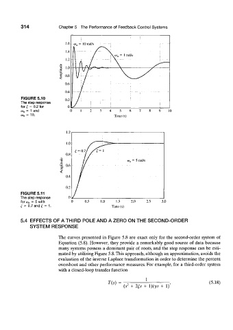
FIGURE 5.10 0.2 i 1
The step response /: -f ^
for l = 0.2 for 0 ' i
oj n = 1 and 4 5 6 10
u> n = 1 0 . Time (s)

1.0
^ = OJ/ /f=l
0.8
alitude p <w„ = 5 rad/s

1
0.4

0.2
FIGURE 5.11
The step response 0
for a) n = 5 with 0.5 1.0 1.5 2.0 2.5 3.0
£ = 0.7 and (= 1. Time (s)

5.4 EFFECTS OF A THIRD POLE AND A ZERO ON THE SECOND-ORDER
SYSTEM RESPONSE

The curves presented in Figure 5.8 are exact only for the second-order system of
Equation (5.8). However, they provide a remarkably good source of data because
many systems possess a dominant pair of roots, and the step response can be esti-
mated by utilizing Figure 5.8. This approach, although an approximation, avoids the
evaluation of the inverse Laplace transformation in order to determine the percent
overshoot and other performance measures. For example, for a third-order system
with a closed-loop transfer function

1
T(s) (5.18)
(r + 2£s + l)(ys + 1)