Page 347 - Modern Control Systems

Section 5.5 The s-Plane Root Location and the Transient Response 321

poles and zeros of T(s) that determine the transient response. However, for a
closed-loop system, the poles of T(s) are the roots of the characteristic equation
A (s) = 0 and the poles of 2P;(.s) A,-(.?). The output of a system (with gain = 1)
without repeated roots and a unit step input can be formulated as a partial fraction
expansion as
A/ Ai N B ks + Q.
Y(s) = - + 2 + 2 l (5.21)
t=i s + cr t £=\ s + 2a ks + (a% + w|)
where the A h B k, and Q. are constants. The roots of the system must be either
.y = —ai or complex conjugate pairs such as s = —a k ± j<o k. Then the inverse trans-
form results in the transient response as the sum of terms
M N
y(t) = l + 2>; e-rv + S V ^ i ^ + **). (5.22)
/=1 k=\
where D k is a constant and depends on B k, C k, a k, and o> k. The transient response is
composed of the steady-state output, exponential terms, and damped sinusoidal
terms. For the response to be stable—that is, bounded for a step input—the real part
-
of the roots, —a/ and -a k, must be in the left-hand portion of the .s-plane. The im-
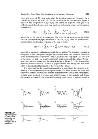
pulse response for various root locations is shown in Figure 5.17. The information
imparted by the location of the roots is graphic indeed, and usually well worth the
effort of determining the location of the roots in the 5-plane.
It is important for the control system analyst to understand the complete rela-
tionship of the complex-frequency representation of a linear system, the poles and
zeros of its transfer function, and its time-domain response to step and other inputs.
In such areas as signal processing and control, many of the analysis and design
calculations are done in the complex-frequency plane, where a system model is

A A A

A A

FIGURE 5.17
Impulse response
for various root ^r- -A- -A- -A-
locations in the 1
s-plane. (The
conjugate root is 0
not shown.)