Page 297 - Orlicky's Material Requirements Planning

276 PART 3 Managing with the MRP System

has its unique challenges. An implementation success strategy for project-driven compa-
nies is discussed in Chapter 16.

MAKE TO STOCK

Make-to-stock companies typically ship to customers on demand. The customers are not
willing to wait very long for their needs to be fulfilled. They expect the products they want
to be on the shelf, typically in a retail environment. Since manufacturing has to build prod-
ucts in advance of customer demand, the manufacturing schedule typically is driven by a
demand forecast. Actual customer demand then consumes this forecast. Ideally, the sales
force will sell to the available to promise (ATP). ATP is the uncommitted portion of invento-
ry. ATP assumes that the plan will be executed as designed and provides visibility on how
much inventory will be available for customer orders. Figure 15-3 provides an example of
ATP.
Available to promise is calculated only in the first time period and whenever there
is an expected receipt. The demand time fence is the expected time within which no addi-
tional customer orders are expected. The demand time fence typically is the length of
time that the customer is expecting to wait for the product he or she has ordered to be
shipped. Within the demand time fence, the actual customer demand is used to calculate
the projected available balance. Once the planning horizon goes beyond the demand time
fence, the projected available balance uses the greater of the forecast or the customer
order. The available-to-promise line uses only confirmed customer demand. Available to
promise is the uncommitted portion of inventory. This is why it is calculated only for the
first time period and whenever there is an expected receipt. Another way to think about
it is how long does the inventory need to last given the current customer backlog.
Cumulative ATP shows how many pieces are available between receipts that have
not been committed already. In some cases, there may be insufficient inventory to cover
the demands that are already known in period 2 until the next receipt in period 4. This is
when a process known as backward ATP is used to reserve that inventory to ensure that
the known customer orders will be covered. In Figure 15-3, the real ATP in period 1
should be 47 pieces. If all 92 pieces are committed to a customer, then the customer’s

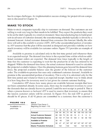
FIGURE 15-3 Part A
Demand Time Fence: 3
Available to Beginning On Hand – 172
promise.
1 2 3 4 5 6 7 8 9 10
Forecast 100 90 80 75 80 90 100 100 120 130
Actual Customer Demand 80 120 75 30 20 10 0 0 0 0
Project Available Balance 92 122 47 122 42 102 2 52 82 102
Available to Promise 92 –45 120
Cumulative ATP 92 47 47 167 167 167 167 167 167 167
Master Production Schedule 150 150 150 150 150 150