Page 156 - PRINCIPLES OF QUANTUM MECHANICS as Applied to Chemistry and Chemical Physics

5.3 Application to orbital angular momentum 147

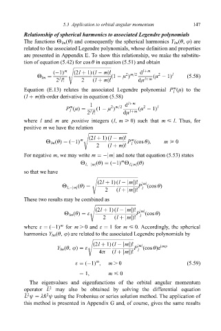
Relationship of spherical harmonics to associated Legendre polynomials
The functions È lm (è) and consequently the spherical harmonics Y lm (è, j) are
related to the associated Legendre polynomials, whose de®nition and properties
are presented in Appendix E. To show this relationship, we make the substitu-
tion of equation (5.42) for cos è in equation (5.51) and obtain
s 
(ÿ1) m (2l ‡ 1) (l ÿ m)! 2 m=2 d l‡m 2 l
È lm ˆ (1 ÿ ì ) (ì ÿ 1) (5:58)
2 l! 2 (l ‡ m)! dì l‡m
l
m
Equation (E.13) relates the associated Legendre polynomial P (ì) to the
l
(l ‡ m)th-order derivative in equation (5.58)
1 d l‡m
m 2 m=2 2 l
P (ì) ˆ 2 l! (1 ÿ ì ) dì l‡m (ì ÿ 1)
l
l
where l and m are positive integers (l, m > 0) such that m < l. Thus, for
positive m we have the relation
s 
(2l ‡ 1) (l ÿ m)!
m
È lm (è) ˆ (ÿ1) m P (cos è), m > 0
2 (l ‡ m)! l
For negative m, we may write m ˆÿjmj and note that equation (5.53) states
m
È l,ÿjmj (è) ˆ (ÿ1) È l,jmj (è)
so that we have
s 
(2l ‡ 1) (l ÿjmj)!
È l,ÿjmj (è) ˆ P jmj (cos è)
2 (l ‡jmj)! l
These two results may be combined as
s 
(2l ‡ 1) (l ÿjmj)!
È lm (è) ˆ å P jmj (cos è)
2 (l ‡jmj)! l
m
where å ˆ (ÿ1) for m . 0 and å ˆ 1 for m < 0. Accordingly, the spherical
harmonics Y lm (è, j) are related to the associated Legendre polynomials by
s 
(2l ‡ 1) (l ÿjmj)!
Y lm (è, j) ˆ å P (cos è)e imj
jmj
4ð (l ‡jmj)! l
m
å ˆ (ÿ1) , m . 0 (5:59)
ˆ 1, m < 0
The eigenvalues and eigenfunctions of the orbital angular momentum
^ 2
operator L may also be obtained by solving the differential equation
^ 2 2
L ø ˆ ë" ø using the Frobenius or series solution method. The application of
this method is presented in Appendix G and, of course, gives the same results