Page 118 - Phase-Locked Loops Design, Simulation, and Applications

MIXED-SIGNAL PLL ANALYSIS Ronald E. Best 77

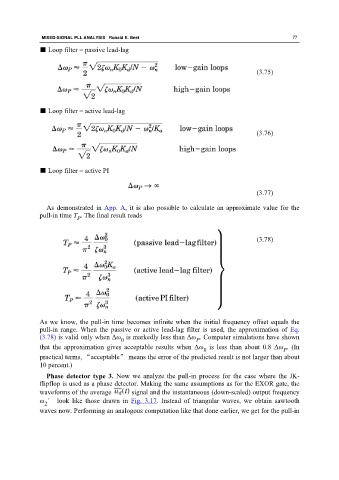
■ Loop filter = passive lead-lag

(3.75)

■ Loop filter = active lead-lag

(3.76)

■ Loop filter = active PI

(3.77)

As demonstrated in App. A, it is also possible to calculate an approximate value for the
pull-in time T . The final result reads
P

(3.78)

As we know, the pull-in time becomes infinite when the initial frequency offset equals the
pull-in range. When the passive or active lead-lag filter is used, the approximation of Eq.
(3.78) is valid only when Δω is markedly less than Δω . Computer simulations have shown
P
0
that the approximation gives acceptable results when Δω is less than about 0.8 Δω . (In
0 P
practical terms, “acceptable” means the error of the predicted result is not larger than about
10 percent.)

Phase detector type 3. Now we analyze the pull-in process for the case where the JK-
flipflop is used as a phase detector. Making the same assumptions as for the EXOR gate, the
waveforms of the average signal and the instantaneous (down-scaled) output frequency
ω ′ look like those drawn in Fig. 3.17. Instead of triangular waves, we obtain sawtooth
2
waves now. Performing an analogous computation like that done earlier, we get for the pull-in