Page 323 - Pipeline Risk Management Manual Ideas, Techniques, and Resources

14/300 Absolute Risk Estimates
the corrosion threat. This unmanaged risk situation might not rect operations survival). Replacing the ANDs with multiplica-
be apparent unless individual index scores are inspected. This is tion signs provides the relationship for probability of survival.
also an important determination if index sums are to be used to Subtracting this resulting product of multiplication from one
infer actual failure probabilities. (1 .O) gives the probability of failure. Because the index scores
The conversion ofinden sum scores into what will be called a are not calibrated to actual survival rates, the probability of fail-
“failure probability score” eliminates the need for any extra ure is a relative score rather than an actual probability. This does
examination of individual index scores. The failure probability not detract from its usefulness as a measurement for decision
scores are calculated from index sum scores by using simple support in matters ofrelative risk.
probability theory. The first step is to assume that each index The conversion to a failure probability score as described
sum represents a survival probability, expressed as a percentage here might be appropriate if a correlation to actual failure rates
chance that the segment will survive for some predetermined is sought or just as a convenience in using relative risk assess-
time period. For example, a corrosion index of 65 indicates that ment results with a scale of “increasing points = increasing
the segment has a 65% chance of survival and 35% chance of safety.” See Chapter 2 for a discussion of the relative merits of
failure in some time period and by some definition of “failure.” either scaling choice.
These percentages are not exact because the index sum is a rela-
tive indicator. However, higher index sums do indicate lower More complex relationships
threats and accompanying higher survivability rates, so some
proportionality does exist. Using the simple percentage rela- The probability of failure tends towards zero when any of four
tionship serves the purpose here. possible scenarios exist:
The failure probability score is obtained by calculating the
probability that the pipeline section will survive all four failure No failure mechanisms exist
modes. Subtracting this probability from 1 .O results in the rela- Failure mechanisms are mitigated-a threat exists but is pre-
tive chance that the pipeline section will fail by any one of the vented from acting on the system. For instance, a high depth
failure modes. This process is illustrated by the following for- of cover or concrete slab protects a pipeline from third-party
mula: damage.
The system is designed for the threat-a failure mechanism
Failure probability score = 1 - (1111 00 x 12/100 x 13/100 x 141100) acts on but cannot harm the system. For example, a pipeline
with sufficient structural strength to resist a slow-acting land
where I1 through 14 are the four indexes representing the failure movement.
mechanisms measured in this risk model. The time-to-failure from a failure mechanism is always
This relationship captures the effects of serious deficiencies greater than the time to detect and correct system weak-
in any one index-representing a very active failure mecha- nesses. For instance, cracks and corrosion flaws can be
nism-ven if the other indexes are presenting a relatively detected and removed while they are still of a size to have no
favorable risk picture. For example, the two scenarios shown in impact on pipeline integrity.
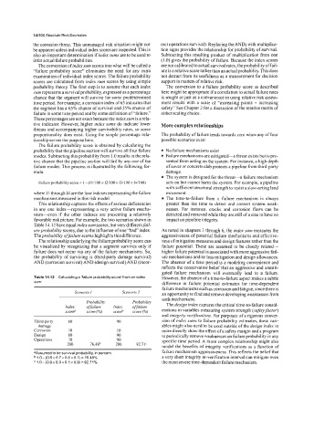
Table 14.12 have equal index sum scores, but very differentfuif-
urepvobability scores, due to the influence of one “bad” index. As noted in chapters 3 through 6, the index sum measures the
The probability offailure scores highlights this difference. aggressiveness of potential failure mechanisms and effective-
The relationship underlying the failure probability score can ness of mitigation measures and design features rather than the
be visualized by recognizing that a segment survives only if failure potential. These are assumed to be closely related-
failure does not occur via any of the failure mechanisms. So, higher failure potential is associated with more aggressive fail-
the probability of surviving is (third-party damage survival) ure mechanisms and/or less mitigation and design allowances.
AND (corrosion survival) AND (design survival) AND (incor- The absence of a time period is a modeling convenience and
reflects the conservative belief that an aggressive and unmiti-
gated failure mechanism will eventually lead to a failure.
Table 14.12 Calculating a ‘failure probability score’ from an index However, the absence of a time-to-failure aspect makes a subtle
sum difference in failure potential estimates for time-dependent
failure mechanisms such as corrosion and fatigue, since there is
Scenario I Scenario 2 an opportunity to find and remove developing weaknesses from
such mechanisms.
Probabilip Probability
Index offailure Index offailure The design index captures the critical time-to-failure consid-
scorea score (%) scot@ score (%) erations in variables measuring system strength (sufetyfactor)
and integriv verzjkutions. For purposes of a rigorous conver-
Third-party 60 90 sion of index sums to failure probability estimates, these van-
damage ables might also need to be used outside of the design index to
Corrosion 70 10 more directly show the effect of a safety margin and a program
Design 80 90 to periodically remove weaknesses on failure probability in any
Operations 70 90 specific time period. A more complex relationship might also
280 76.4Sb 280 92.7lC
model the benefits of integrity verifications as a function of
aAssumed lo be survival probability, in percent failure mechanism aggressiveness. This reflects the belief that
1.0- (0.6~ 0.7x0.8 x 0.7) = 76.48%. a very short integrity re-verification interval can mitigate even
1 .O - (0.9 0.9 x 0.1 x 0.9) = 92.71 %. the most severe time-dependent failure mechanism.
x