Page 371 - Pipeline Risk Management Manual Ideas, Techniques, and Resources

15/36 Risk Management
L, variables. A costirisk mathematical relationship can be theo-
rized for each mitigation activity. For most management deci-
sions, this relationship need not be highly precise. The user is
usually interested in comparing the cost of equivalent risk-
reducing alternatives. When costs of alternatives are close, fur-
ther refinement of costs may be required; however, the costs
of many of the possible options will be orders of magnitude
dfferent.
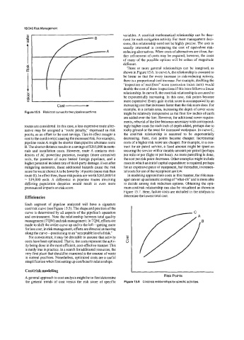
Three or more general relationships can be imagined, as
shown in Figure 15.6. In curve A, the relationship is assumed to
be linear so that for every increase in risk-reducing activity,
there is a proportional cost increase. For example, doubling the
“inspection of rectifiers” score (corrosion index item) would
double the cost of those inspections if this item follows a linear
cost - be exponentially increasing. In this case, risk points become
relationship. In curve B, the cost‘risk relationship is assumed to
more expensive: Every gain in risk score is accompanied by an
increasing cost that increases faster than the risk score does. For
example, in a certain area, increasing the depth of cover score
Figure 15.5 Risklcost curves for two pipeline sections. might be relatively inexpensive as the first few inches of earth
are added over the line. However, for additional cover require-
ments, reburial of the line becomes necessary with correspond-
routes are considered. In this case, a less expensive route alter- ingly higher costs for each inch of depth added, perhaps due to
native may be assigned a “route penalty,” expressed in risk rocky ground or the need for increased workspace. In curve C,
points, as an offset to the cost savings. This in effect assigns a the cost‘risk relationship is assumed to be exponentially
cost to the condition(s) causing the increased risk. For example, decreasing. Here, risk points become cheaper: Incremental
pipeline route A might be shorter than pipeline alternate route costs of a higher risk score are cheaper. For example, in a con-
B. The shorter distance results in a savings of $265,000 in mate- tract for air patrol service, a fixed amount might be spent on
rials and installation costs. However, route A contains inci- securing the service with a variable amount per patrol (perhaps
dences of AC powerline presence, swampy (more corrosive) per mile or per flight or per hour). As more patrolling is done,
soils, the presence of more buried foreign pipelines, and a the cost per risk point decreases. Other examples might include
higher potential incident rate of third-party damage. Even after cases in which an initial capital expenditure is required, perhaps
mitigating measures, these additional hazards cause the risk for an expensive piece of equipment, but thereafter, incremen-
score for route choice A to be lower by 14 points (more risk than tal costs for use of the equipment are low.
route B). In effect then, those risk points are worth $265,000/14 In modeling approximate costs in this manner, the risk man-
= $19,000 each. A difference in pipeline routes involving ager can set up automatic costing of “what-ifs” and is more able
differing population densities would result in even more to decide among risk reduction options. Obtaining the opti-
pronounced impacts on risk score. mum cost‘risk relationship can also be visualized as shown in
Figure 15.7. Here, failure costs are included in the analysis to
Efficiencies determine the lowest total cost.
Each segment of pipeline analyzed will have a signature
costirisk curve (see Figure 15.5). The shape and position of the
curve is determined by all aspects of the pipeline’s operation
and environment. Note the relationship between total quality
management (TQM) and riskmanagement: InTQM, efforts are
made to shift the entire curve up and to the left-getting more
for less cost; in risk management, efforts are directed at moving
along the curve-positioning to an “acceptable level of risk.”
For convenience, it may be desirable to assume that activity
costs have been optimized. That is, the costs represent the activ-
ity being done in the most efficient, cost-effective manner. This
is rarely trve in practice. In a search for additional resources, the
very first place that should be examined is the amount of waste
in current practices. Nonetheless, optimized costs are a useful
simplification when first setting up costhenefit relationships.

Costkisk modeling I
Risk Points
A general approach to cost analysis might be to first determine
the general trends of cost versus the risk score of specific Figure 15.6 CosWrisk relationships for specific activities.