Page 99 - Power Electronic Control in Electrical Systems

//SYS21/F:/PEC/REVISES_10-11-01/075065126-CH003.3D ± 87 ± [82±105/24] 17.11.2001 9:53AM

Power electronic control in electrical systems 87

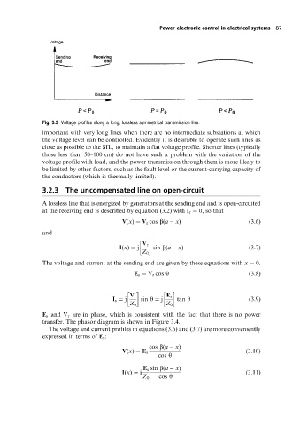
Fig. 3.3 Voltage profiles along a long, lossless symmetrical transmission line.
important with very long lines when there are no intermediate substations at which
the voltage level can be controlled. Evidently it is desirable to operate such lines as
close as possible to the SIL, to maintain a flat voltage profile. Shorter lines (typically
those less than 50±100 km) do not have such a problem with the variation of the
voltage profile with load, and the power transmission through them is more likely to
be limited by other factors, such as the fault level or the current-carrying capacity of
the conductors (which is thermally limited).

3.2.3 The uncompensated line on open-circuit

A lossless line that is energized by generators at the sending end and is open-circuited
at the receiving end is described by equation (3.2) with I r ˆ 0, so that
V(x) ˆ V r cos b(a x) (3:6)

and

V r
I(x) ˆ j sin b(a x) (3:7)
Z 0
The voltage and current at the sending end are given by these equations with x ˆ 0.
E s ˆ V r cos y (3:8)

V r E s
I s ˆ j sin y ˆ j tan y (3:9)
Z 0 Z 0
E s and V r are in phase, which is consistent with the fact that there is no power
transfer. The phasor diagram is shown in Figure 3.4.
The voltage and current profiles in equations (3.6) and (3.7) are more conveniently
expressed in terms of E s :
cos b(a x)
V(x) ˆ E s (3:10)
cos y
E s sin b(a x)
I(x) ˆ j (3:11)
Z 0 cos y