Page 103 - Power Electronic Control in Electrical Systems

//SYS21/F:/PEC/REVISES_10-11-01/075065126-CH003.3D ± 91 ± [82±105/24] 17.11.2001 9:53AM

Power electronic control in electrical systems 91

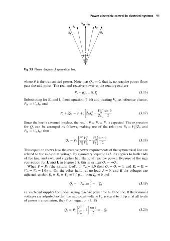
Fig. 3.9 Phasor diagram of symmetrical line.

where P is the transmitted power. Note that Q m ˆ 0, that is, no reactive power flows
past the mid-point. The real and reactive power at the sending end are
P s ‡ jQ s ˆ E s I s (3:16)

Substituting for E s and I s from equation (3.14) and treating V m as reference phasor,
P m ˆ V m I m and
V 2 sin y
2 m
P s ‡ jQ s ˆ P ‡ jZ 0 I (3:17)
m
Z 0 2
Since the line is assumed lossless, the result P ˆ P s ˆ P r is expected. The expression
2
for Q s can be arranged as follows, making use of the relations P 0 ˆ V /Z 0 and
0
P m ˆ V m I m : thus
2 2 2
P V 0 V m sin y
Q s ˆ P 0 (3:18)
2
P V 2 V 2 2
0 m 0
This equation shows how the reactive power requirements of the symmetrical line are
related to the mid-point voltage. By symmetry, equation (3.18) applies to both ends
of the line, and each end supplies half the total reactive power. Because of the sign
convention for I s and I r in Figure 3.8, this is written Q s ˆ Q r .
When P ˆ P 0 (the natural load), if V m ˆ 1:0 then Q s ˆ Q r ˆ 0, and E s ˆ E r ˆ
V m ˆ V 0 ˆ 1:0p:u: On the other hand, at no-load P ˆ 0, and if the voltages are
adjusted so that E s ˆ E r ˆ V 0 ˆ 1:0p:u:, then I m ˆ 0 and

y
Q s ˆ P 0 tan ˆ Q r (3:19)
2
i.e. each end supplies the line-charging reactive power for half the line. If the terminal
voltages are adjusted so that the mid-point voltage V m is equal to 1.0 p.u. at all levels
of power transmission, then from equation (3.18)

2
P sin y
Q s ˆ P 0 2 1 ˆ Q r (3:20)
P 0 2