Page 104 - Power Electronic Control in Electrical Systems

//SYS21/F:/PEC/REVISES_10-11-01/075065126-CH003.3D ± 92 ± [82±105/24] 17.11.2001 9:53AM

92 Transmission system compensation

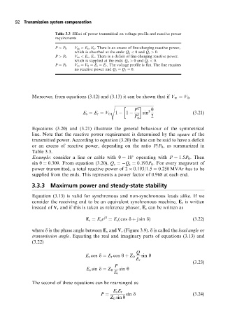
Table 3.3 Effect of power transmitted on voltage profile and reactive power
requirements

P < P 0 V m > E s , E r . There is an excess of line-charging reactive power,
which is absorbed at the ends: Q s < 0 and Q r > 0.
P > P 0 V m < E s , E r . There is a deficit of line-charging reactive power,
which is supplied at the ends: Q s > 0 and Q r < 0.
P ˆ P 0 V m ˆ V 0 ˆ E s ˆ E r . The voltage profile is flat. The line requires
no reactive power and Q s ˆ Q r ˆ 0.

Moreover, from equations (3.12) and (3.13) it can be shown that if V m ˆ V 0 ,

s 
P 2 y
2
E s ˆ E r ˆ V 0 1 1 2 sin (3:21)
P 2
0
Equations (3.20) and (3.21) illustrate the general behaviour of the symmetrical
line. Note that the reactive power requirement is determined by the square of the
transmitted power. According to equation (3.20) the line can be said to have a deficit
or an excess of reactive power, depending on the ratio P/P 0 , as summarized in
Table 3.3.
Example: consider a line or cable with y ˆ 18 operating with P ˆ 1:5P 0 . Then

sin y ˆ 0:309. From equation (3.20), Q s ˆ Q r ˆ 0:193P 0 . For every megawatt of
power transmitted, a total reactive power of 2 0:193/1:5 ˆ 0:258 MVAr has to be
supplied from the ends. This represents a power factor of 0.968 at each end.

3.3.3 Maximum power and steady-state stability

Equation (3.13) is valid for synchronous and non-synchronous loads alike. If we
consider the receiving end to be an equivalent synchronous machine, E r is written
instead of V r and if this is taken as reference phasor, E s can be written as
jd
E s ˆ E s e ˆ E s ( cos d ‡ j sin d) (3:22)

where d is the phase angle between E s and V r (Figure 3.9). d is called the load angle or
transmission angle. Equating the real and imaginary parts of equations (3.13) and
(3.22)
Q
E s cos d ˆ E r cos y ‡ Z 0 sin y
E r
(3:23)
P
E s sin d ˆ Z 0 sin y
E r
The second of these equations can be rearranged as

E s E r
P ˆ sin d (3:24)
Z 0 sin y