Page 109 - Practical Control Engineering a Guide for Engineers, Managers, and Practitioners

84 Chapter Four

2 .·
iC
.
.
.
~ . . . . . . . . . . . . . . .
Q.l 1.5
"'0
.a
-~ 1
!U
~ 0.5
0 0.05 0.1 0.15 0.2 0.25 0.3 0.35 0.4 0.45 0.5
(A)
0.---.---.---.---~--.----r---.--~---.--~
- -20 . . . . . ..
0
i -40 ..
f -60 .· ..... ·. . . . . . . . ..
. . . .......
~o~~~~==~~====~~~~d
0 0.05 0.1 0.15 0.2 0.25 0.3 0.35 0.4 0.45 0.5
Frequency (/min)
(B)
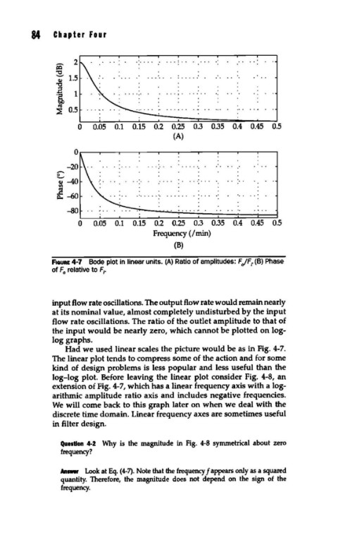
F•auRE 4-7 Bode plot in linear units. (A) Ratio of amplitudes: F JFr (B) Phase
of F relative to F•
0 1

input flow rate oscillations. The output flow rate would remain nearly
at its nominal value, almost completely undisturbed by the input
flow rate oscillations. The ratio of the outlet amplitude to that of
the input would be nearly zero, which cannot be plotted on log-
log graphs.
Had we used linear scales the picture would be as in Fig. 4-7.
The linear plot tends to compress some of the action and for some
kind of design problems is less popular and less useful than the
log-log plot. Before leaving the linear plot consider Fig. 4-8, an
extension of Fig. 4-7, which has a linear frequency axis with a log-
arithmic amplitude ratio axis and includes negative frequencies.
We will come back to this graph later on when we deal with the
discrete time domain. Linear frequency axes are sometimes useful
in filter design.

Question 4-2 Why is the magnitude in Fig. 4-8 symmetrical about zero
frequency?

AniWII' Look at Eq. (4-7). Note that the frequency Jappears only as a squared
quantity. Therefore, the magnitude does not depend on the sign of the
frequency.