Page 107 - Practical Control Engineering a Guide for Engineers, Managers, and Practitioners

82 Chapter Four

and the phase is the angle whose tangent is the ratio of the imaginary
to the real part

1
-
6=tan- 1 - -r2nf) =-tan- (r2nf) (4-8)
( 1
The last two equations tum out to be the same as Eq. (4-5). So, we
see one more reason why the Laplace transform can be so useful:
there is an easy, straightforward path from the Laplace domain to the
frequency domain. All you have to do is accept the serendipitous
effect of replacing the Laplace operator by jm. There is one caveat.
The result of making the substitution gives the steady-state sinusoidal
solution after the transients have died out-remember, when you
feed a sinusoid to a process, the process output requires some time to
evolve toward a sinusoidal function. Refer to App. B where the full
solution, including the transient part, is given.

4·1·4 A Uttle Graphical Support
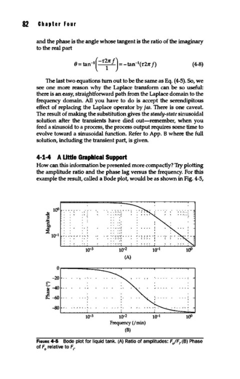
How can this information be presented more compactly? Try plotting
the amplitude ratio and the phase lag versus the frequency. For this
example the result, called a Bode plot, would be as shown in Fig. 4-5,

tOO -· ·---- - - --....
: I ~ I o o\lo! I I I o o ~

0 0 ., ... ;
·-·~ .. •.1- ••• ..................
,, •••
0 0 0 ; ~ 0 i ~ ; ; 0 i ~
0 0 ,\ I
10-3 10-2 10-1
(A)
0
-20 •••• l
0"
i-40
fir
f-60
-80 ....... ·".
10-3 10-2 10-1 100
Frequency (/min)
(8)
F1auRE 4-6 Bode plot for liquid tank. (A) Ratio of amplitudes: F JFr (B) Phase
of F relative to F •
0 1