Page 137 - Practical Control Engineering a Guide for Engineers, Managers, and Practitioners

112 Chapter Four

0.7
0.6 . . . ...
0.5
0.4
:::s
0.3 ..
0.2
0.1
0
0 10 20 30 40 50 60 70 80 90 100

2
1.5
V)
"'0
c:: 1 -·-·- --·
<U
>-

40 50 60 70 80 90 100
Time

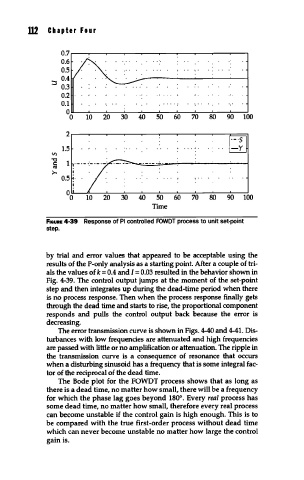
F•auRE 4-39 Response of PI controlled FOWDT process to unit set-point
step.

by trial and error values that appeared to be acceptable using the
results of the P-only analysis as a starting point. After a couple of tri-
als the values of k = 0.4 and I= 0.03 resulted in the behavior shown in
Fig. 4-39. The control output jumps at the moment of the set-point
step and then integrates up during the dead-time period when there
is no process response. Then when the process response finally gets
through the dead time and starts to rise, the proportional component
responds and pulls the control output back because the error is
decreasing.
The error transmission curve is shown in Figs. 4-40 and 4-41. Dis-
turbances with low frequencies are attenuated and high frequencies
are passed with little or no amplification or attenuation. The ripple in
the transmission curve is a consequence of resonance that occurs
when a disturbing sinusoid has a frequency that is some integral fac-
tor of the reciprocal of the dead time.
The Bode plot for the FOWDT process shows that as long as
there is a dead time, no matter how small, there will be a frequency
for which the phase lag goes beyond 180°. Every real process has
some dead time, no matter how small, therefore every real process
can become unstable if the control gain is high enough. This is to
be compared with the true first-order process without dead time
which can never become unstable no matter how large the control
gain is.