Page 258 - Radar Technology Encyclopedia

loss, atmospheric (attenuation) loss, beamshape 248

3000
R = ------------------------------------------------ m
a – 4
æ 2.5 ´ 10 ö
+
sin q ------------------------
è q 0.028+ ø
is the effective sea-level pathlength. Frequency dependence is
accounted for by the coefficient k , shown in Table L7.
a
If part of the path R is occupied by precipitation, there
pr
will be an additional loss:
R pr ö
L ( R , ) k apr a exp æ – -------- (dB)
R 1 –
q =
a
R ø
è
pr
a
where k apr is the precipitation attenuation coefficient shown
in the table. The total attenuation will include that of the air
and the embedded precipitation:
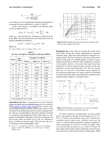
Figure L18 Atmospheric lens loss (two-way) vs. range, for dif-
L R q,( ) L ( R q, ) L ( R q, ) (dB)
=
+
a a apr ferent elevation angles (after Weil).
DKB, SAL
Ref.: Blake (1980), pp. 197–221; Barton (1993), p. 113.
Beamshape loss is the result of covering the search sector
Table L7
with beams having the typical (approximately Gaussian)
Two-Way Atmospheric Attenuation Coefficients (dB/km)
mainlobe shape, rather than with (idealized) contiguous rect-
Atmospheric conditions angular beams. This loss is defined as the ratio of echo power
Freq.
Band required at the peak of a scanning pattern, to achieve a given
(GHz)
Clear, k a Rain, k /r Snow, k /r detection performance when the signal integration is matched
a
a
to that pattern, relative to the power that would have been
UHF 0.4 0.01 0 0
required for a uniform signal envelope existing over the time
L 1.3 0.012 0.0003 0.0003
required to scan one beamwidth (Fig. L19). For a two-coordi-
S 3.0 0.015 0.0013 0.0013 nate scan, it is the ratio of transmitted energy required for
given detection performance for targets uniformly distributed
C 5.5 0.017 0.008 0.008
over the search solid angle to the energy that would have been
X 10 0.024 0.037 0.002
required using contiguous, rectangular beams.
Ku 15 0.055 0.083 0.004
Continuous scan Voltage
K 22 0.30 0.23 0.008
1.0 G G r
t
0.8
Ka 35 0.14 0.57 0.015
Scan 0.6 p L
V 60 35 1.3 0.03 0.4 t o
t
G G r f t (q) f r (q)
0.2
W 95 0.80 2 0.06
0 Time
140 1.0 2.3 0.06
Discrete scan Voltage
240 15 2.2 0.08 1.0 G G r
t
0.8
r is the precipitation rate in mm/h 0.6 G G r f (q,f) (q,f)
f
t
r
t
0.4 p L (averaged over two-
Atmospheric lens loss is a propagation loss at low elevation 0.2 coordinate angle space)
angles, in which rays are refracted downward (according to 0 Time
the 4/3 effective earth’s radius model, under normal condi-
tions), diluting the power density at the target relative to that Figure L19 Definition of beamshape loss for one-coordinate
continuous scan and discrete-position raster scan.
calculated from antenna gain and free-space propagation the-
ory. The loss is nondissipative, and hence should be included
For both continuously scanning beams and step-scanned
as a reduction in the propagation factor, rather than as a com-
beams with optimum spacing, the beamshape loss for P »
ponent of atmospheric attenuation. The loss is reciprocal, and d
0.5 is 1.23 dB for one-coordinate scans, and 2.5 dB for two-
the two-way values are shown in Fig. L18, As a function of
coordinate (raster or spiral) scans. (In Blake’s early work, the
range, for different elevation angles. The term lens-effect loss
value of 1.6 dB included nonoptimum integrator weighting as
is sometimes used interchangeably. DKB
well as beamshape loss.) The loss increases for higher values
Ref.: Weil, T. A., “Atmospheric Lens Effect: Another Loss for the Radar
of P , because the increased P (e.g., from 0.9 toward 1.0)
Equation,” IEEE Trans. AES-9, no. 1, Jan. 1973, pp. 51–54; Blake d d
(1980), p. 188. near centers of the beams cannot compensate for the decrease
(e.g, from 0.9 toward 0) near the beam-overlap regions. When