Page 260 - Radar Technology Encyclopedia

loss, blind-phase loss, collapsing 250

the number of degrees of freedom for both signal and noise is
reduced from two to one per pulse (the distributions are
changed from Rayleigh to Gaussian). Unless the processor
integrates over a period long enough to receive both compo-
nents of a fluctuating signal, the fluctuation loss (in decibels)
is doubled, a serious factor for high values of P (see Fig.
d
L26). The increase in fluctuation loss is the blind phase loss.
DKB
Ref.: Barton (1988), p. 251; Nathanson (1991), p. 393.
A loss budget is a listing of all loss factors applicable to a
given radar system operating in a given mode and environ-
ment. The loss should be divided into the four classes shown
in Tables L2 to L5 to permit proper values to be used in dif-
ferent forms of the radar equation. A typical loss budget,
applicable to a short-range search radar using MTI, is shown
in Table L8. DKB
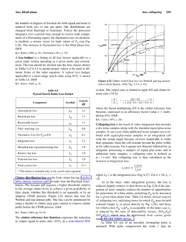
Figure L22 Clutter distribution loss for Weibull and log-normal
Ref.: Barton (1988), p. 28.. clutter (from Barton, 1988, Fig. 2.5.4, p. 93).

Table L8 system. The output ratio is related to input S/N and clutter-to-
Typical Search Radar Loss Budget noise ratio C/N by
¤
(
æ S ö 2 CN ) æ S ö
Loss in ------ = ------------------------------------------------------- ------
¤ è
Component Symbol è N ø 1 + 2 SN ) 2 CN )N ø
(
¤ +
(
o
dB
where the factor multiplying S/N is the clutter-reference loss
Atmospheric loss L a 1.2 function, expressed as an efficiency factor (value < 1, multi-
plying S/N). DKB
Beamshape loss L p 1.3
Ref.: Currie (1987), p. 266.
Beamwidth factor* 1.2
Ln Collapsing loss is the result of video integration that includes
Filter matching loss L m 0.8 extra noise samples along with the intended signal-plus-noise
samples. It can occur when additional noise samples are com-
Fluctuation loss (for P = 0.9) L f 8.4 bined with signal-plus-noise samples in an integration cell
d
with the actual target because receiver bandwidth is wider
Integration loss L i 3.2 than optimum, when the cell extends beyond the pulse width,
Miscellaneous signal-processing loss L x 3.0 or for other reasons. For a square-law detector followed by an
integrator processing n samples of signal plus noise and m
Receive line loss L r 1.0 additional noise samples, a collapsing ratio is defined as
r=1 + m/n. The collapsing loss is then calculated as the
Transmit line loss L t 1.0 increase in integration loss:
(
Total system loss L s 21.1 L rn )
i
L r n ) ----------------
(
=
c L n ()
* This factor is included only in the search radar equation i
where L (×) is the integration loss (Fig. L27). For n > 10, L »
i
c
Clutter distribution loss results from clutter having a proba- r .
bility density function (pdf) broader than the Rayleigh distri- As in the basic video integration process, the loss is
bution. The broader pdf requires a higher threshold, relative reduced slightly relative to that shown in Fig. L28 if the inte-
to the average clutter level, to achieve a given probability of gration of more samples reduces the number of opportunities
false alarm, whether this threshold is set manually or by an for generation of a false alarm, permitting P to be increased
fa
adaptive CFAR process. Figure L22 shows this loss for for a given false-alarm time. Table L9 shows several sources
Weibull and log-normal pdfs. The loss can be minimized by of collapsing loss, indicating those for which P must be held
fa
using a limiter or clutter map gain control to remove clutter constant (larger L as given directly by Fig. L28), and those
c
peaks before the CFAR process. DKB for which a new P ¢ = rP is acceptable. In the latter case, L c
fa
fa
Ref.: Barton (1988), pp. 92–94 is reduced by the ratio of detectability factors, D(P ,P )/
d
fa
D(P ,P ¢), which may be determined from curves given
d
fa
The clutter-reference loss function expresses the reduction
under DETECTION curves.
in output signal-to-noise ratio (S/N) in a noncoherent MTI In Table L9, use of an uncoded, rectangular pulse is
o
assumed. With pulse compression the value t may be