Page 264 - Radar Technology Encyclopedia

loss, fluctuation loss, integrator weighting 254

correlation time t >> t ). Fluctuation loss also depends Df
o
c
e
slightly on the number of pulses integrated. For n-pulse inte- n = 1 + ----- £ n
f
c
gration, the loss is approximated as
f
where D is the diversity bandwidth, f = c/2L is the target
(
,
log
=
10log L n 1 ) ( 10 + 0.03n ) L 1 () c r
f f correlation frequency, and L is the radial length of the target.
r
Polarization diversity can provide a factor of two increase
in n . DKB
e
Ref.: Barton (1988), p. 84.
Insertion loss refers to the attenuation inserted by a passive
component into a signal path (see ATTENUATION).
Integration loss refers to the loss, relative to ideal (coherent)
integration of signal samples, resulting from integration after
envelope detection. The loss results from the increase in
detector loss as input SNR is reduced and may be calculated
as a function of n, the number of pulse integrated and the
basic, single-pulse detectability factor D (1):
0
9.2nD 1 () 2.3+
0
1 + 1 + ----------------------------------------
2
[ D 1 ()]
0
L n () ---------------------------------------------------------------
=
i
9.2D 1 () 2.3+
0
1 + 1 + ------------------------------------
Figure L26 Fluctuation loss for a slowly fluctuating Rayleigh 2
[ D 1 ()]
(Swerling case 1) target, as a function of detection probability 0
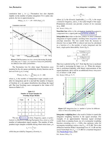
for different false-alarm probabilities. This loss is plotted in Fig. L27. Note that the loss is moderate
for small n, increasing for large n as n . When the integra-
The fluctuation loss for other target fluctuation cases
tion is performed digitally with binary representation of the
modeled by the chi-square probability density function can be
signal amplitude, there will be an additional binary integrator
derived from L (n,1) using
f
loss of about 1.6 dB. DKB
10
,
(
10log L nKn ) ---------log= L n 1 ,( ) (dB) Ref.: Barton (1988), pp. 71–73.
f e Kn e f
15
where n is the number of independent target samples avail- 14
e
able for integration and K is one-half the number of degrees 13
of freedom of a chi-square distribution describing the target 12
pdf. The four Swerling cases correspond to the values of K 11
10
shown in Table L12:. Integration loss, L i , (dB) 9
Table L12 8 7 6 dB 10 dB 12 dB 20 dB
Number of Target Samples for 6 18 dB
Swerling Target Models 5 D 0 (1) = 0 dB 16 dB
4 14 dB
3
Case K n e Kn e 2
1
1 1 1 1 0 1 10 100 1 10 3
Number of pulses, n
2 1 n n
Figure L27 Integration loss vs. number of pulses for different
3 2 1 2 values of basic detectability factor.
4 2 n 2n Integrator weighting loss is the result of failure to match the
integrator weighting function to the signal envelope. For
The use of diversity (in time, frequency, space, or polar-
example, if an approximately Gaussian signal envelope
ization) is effective in reducing fluctuation loss, since n is the results from a scanning beam, use of a rectangular weighting
e
number of independent signal samples. The number of inde-
function extending over t = 0.88t (the optimum value for
o
i
pendent target samples available during observation time t is rectangular weighting) causes a loss L » 0.35 dB. This is the
o
t o iw
n = 1 + ---- £ n difference between Blake’s beamshape loss of 1.6 dB and the
e t
c actual beamshape loss L = 1.25 dB for a matched integrator.
p
while that provided by frequency diversity is (See beamshape loss.) DKB
Ref.: Barton (1988), p. 76.