Page 93 - Rock Mechanics For Underground Mining

THE HEMISPHERICAL PROJECTION

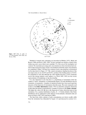
Figure 3.27 Plots of poles of
351 discontinuities (after Hoek and
Brown, 1980).

Methods of manual pole contouring are described by Phillips (1971), Hoek and
Brown (1980) and Priest (1985, 1993). In these methods, the numbers of poles lying
within successive areas which each constitute 1% of the area of the hemisphere are
counted. The maximum percentage pole concentrations are then determined and con-
tours of decreasing percentage of pole concentrations around the major concentrations
are established. Figure 3.28 shows the contours of pole concentrations so determined
for the data shown in Figure 3.27. The central orientations (dip/dip direction) of the
two major joint sets are 22/347 and 83/352, and that of the bedding planes is 81/232.
It is important to note that although the order dip/dip direction is most commonly
used in the mining industry, some authors (e.g. Priest 1985, 1993) use the reverse
representation of trend/plunge or dip direction/dip.
It is also important to note that there is a distribution of orientations about the
central or “mean” orientations. As illustrated by Figure 3.28, this distribution may be
symmetric or asymmetric. A number of statistical models have been used to provide
measures of the dispersion of orientations about the mean. The most commonly used
of these is the Fisher distribution (Fisher, 1953) in which the symmetric dispersion
of data about the mean in represented by a number, K, known as the Fisher constant.
The higher the value of K, the less is the dispersion of values about the mean or true
orientation. For a random distribution of poles, K = 0. Further details of the Fisher
distribution and its application to the analysis of discontinuity orientation data are
given by Priest (1985, 1993) and Brown (2003).
The data from which contours of pole concentrations are drawn usually suffer
from the orientation bias illustrated by Figure 3.13 and discussed in section 3.4.1.
75